Build a map to compare metrics by country or region
If you want to learn Maps by building something, this tutorial takes you from an empty map to a dashboard that shows web traffic by country and by location.
You’ll learn to:
- Create a map with multiple layers and data sources, such as reference boundaries and Elasticsearch data
- Use symbols, colors, and labels to style data values, from choropleth shading to cluster sizes
- Embed a map in a dashboard
- Filter across panels in your dashboard, including from the map itself
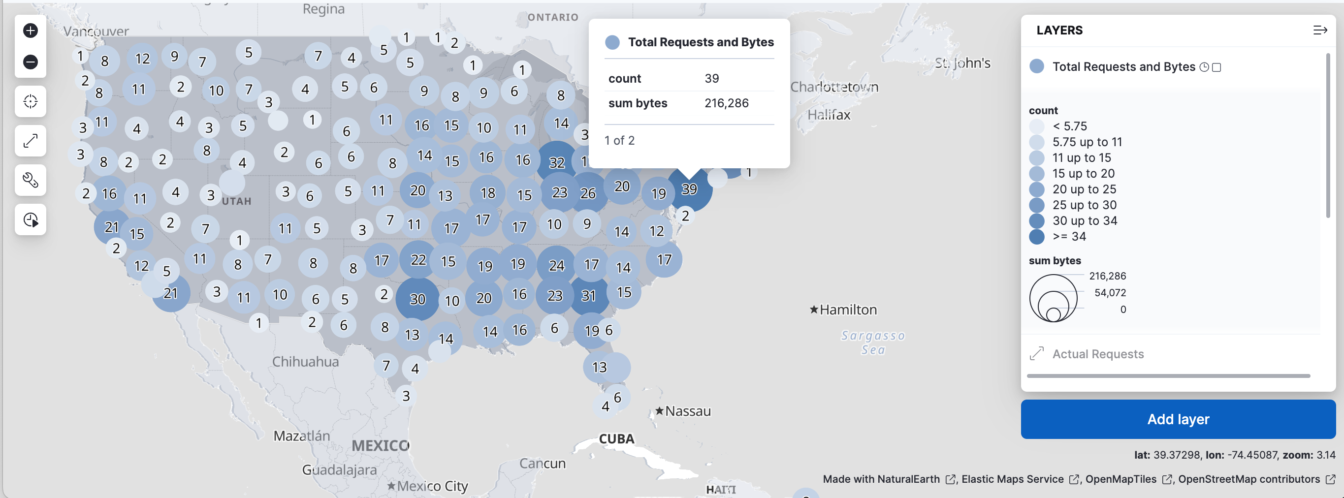
When you complete this tutorial, you’ll have a map like this one:
You don’t need experience with Maps, but you should know how to open and edit a dashboard.
- If you don’t already have Kibana, set it up with our free trial.
- This tutorial requires the web logs sample data set. The sample data includes a [Logs] Total Requests and Bytes map, which you’ll re-create in this tutorial.
- You must have the correct privileges for creating a map. If you don’t have sufficient privileges to create or save maps, a Read only badge appears. For more information, refer to Granting access to Kibana.
You build the map on a dashboard. When you save the map, you return to that dashboard. A map is a stack of layers. The Basemap layer draws the background, and every layer you add draws your data on top of it.
Open the Dashboards page and select Create dashboard.
Set the time range to Last 7 days.
The map and the other panels show only data from this time range. If a panel looks empty later, widen the range.
Add a map panel:
-
Select Add. In the Add to dashboard flyout, select Maps in the Other visualizations group. -
Select Add → New panel, then select Maps in the Visualizations group. -
Select Add panel, then select Maps in the Visualizations group.
The map editor opens. Its Layers panel lists the Basemap layer and has an Add layer button.
-
A choropleth layer shades areas by a value. In this map, a country gets a darker shade the more web log requests it receives. Kibana gets the country shapes from the Elastic Maps Service (EMS), then matches each shape to the web logs by country code. This match is called a join.
Select Add layer, then select Choropleth.
The Add layer panel offers more layer types. This tutorial uses Choropleth, Documents, and Clusters. To learn about the others, refer to Vector layer, Heat map layer, and Tile layer.
To draw the country shapes, keep Boundaries source set to Administrative boundaries from the Elastic Maps Service, then select World Countries in EMS boundaries.
The Join field in this section is ISO 3166-1 alpha-2 code, the two-letter country code, such as
US. Leave it as it is.To count web logs per country, set these options in Statistics source:
- Data view to Kibana Sample Data Logs
- Join field to geo.dest
Kibana counts the web log documents for each value of
geo.dest, the country code of the request’s destination.Select Add and continue.
Kibana adds the layer and opens its settings.
In Layer settings, set:
- Name to
Total Requests by Destination - Opacity to 50%
The name identifies the layer in the layer list, the legend, and tooltips. A lower opacity lets the basemap show through the shaded countries.
- Name to
When you select a country on the map, its tooltip lists the tooltip fields. ISO 3166-1 alpha-2 code is already there. To also show the country name:
- Select Add to open the field list.
- Select name, then select Add.
The
namefield holds the country name from the EMS boundaries, for exampleUnited States of America. Without it, the tooltip shows only the country code and the request count.In Layer style:
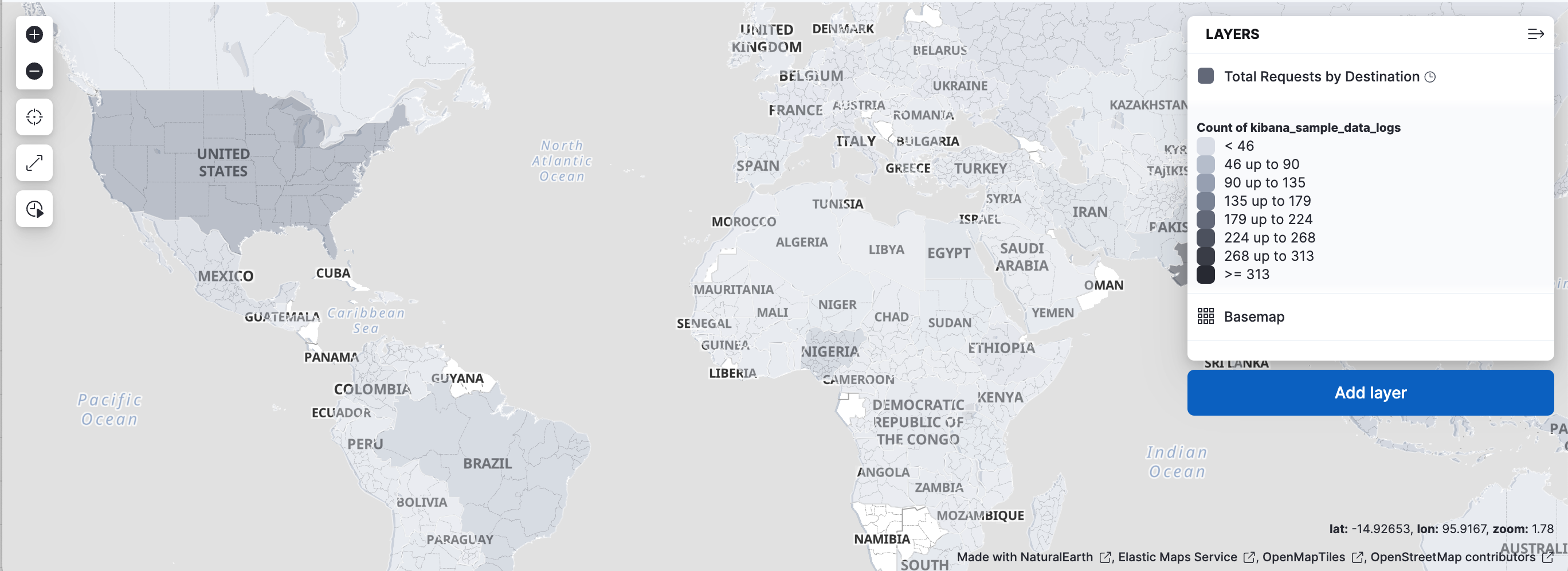
- Set Fill color to As number, then select the gray color ramp. With this ramp, countries with more requests get a darker shade.
- Set Border color to white. White borders separate neighboring countries.
- Under Label, change By value to Fixed. By default, the layer labels each country with its request count. A fixed label with no text removes these labels and leaves the basemap’s country names readable.
To learn more about styling options, refer to Vector style.
Select Keep changes.
Your map now shows the countries shaded by traffic:
On a map of the whole world, a point for every web request would be unreadable. Zoomed in on a street, a cluster would hide the individual requests. To handle both, you’ll add two layers and set the zoom levels where each one is visible: one for individual requests, and one for clusters of requests. Zoom levels run from 0, the whole world, to 24, individual streets.
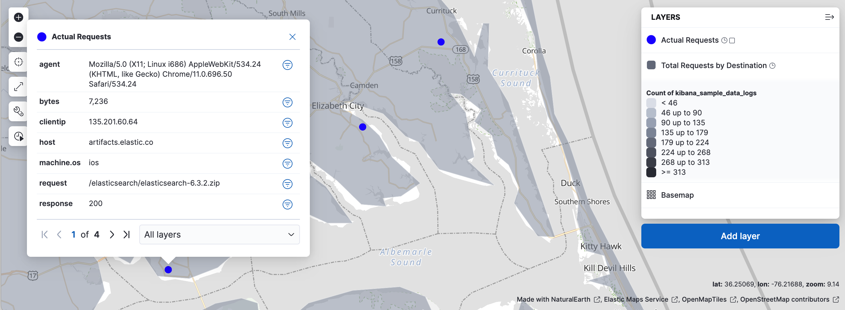
This layer displays each web log document as a point. It’s visible only when you zoom in.
Select Add layer, then select Documents.
Set Data view to Kibana Sample Data Logs.
Geospatial field is already set to geo.coordinates. This field stores the location of each request, and Kibana uses it to place each document on the map. If your data view has more than one geospatial field, this is where you choose which one to plot.
Select Add and continue.
In Layer settings, set:
- Name to
Actual Requests - Visibility to the range [9, 24]
- Opacity to 100%
Visibility limits the layer to zoom levels 9 through 24.
- Name to
Add the tooltip fields to show when you select a point: agent, bytes, clientip, host, machine.os, request, response, and timestamp.
In Scaling, select Limit results to 10,000.
Kibana draws at most 10,000 documents for the visible map area, which keeps the map fast. To compare this option with the others, refer to Vector layer.
In Layer style, set Fill color to #2200FF.
Select Keep changes.
From zoom level 9 to 24, your map shows individual requests:
A clusters layer groups nearby documents into grid cells and draws one circle for each cell. Because it uses an aggregation, the layer stays fast even for very large data sets. You make it visible only when the map is zoomed out. Darker circles mark cells with more web log requests, and larger circles mark cells with more bytes transferred.
Select Add layer, then select Clusters.
Set Data view to Kibana Sample Data Logs.
Geospatial field is again geo.coordinates. It decides which grid cell each document falls into.
Select Add and continue.
In Layer settings, set:
- Name to
Total Requests and Bytes - Visibility to the range [0, 9]
- Opacity to 100%
With the Actual Requests layer, this range means that one of the two layers is visible at every zoom level: clusters from 0 to 9, and individual requests from 9 to 24.
- Name to
In Metrics:
- Keep Aggregation set to Count.
- Select Add metric.
- Set Aggregation to Sum with Field set to bytes.
Each cluster now reports two values: the number of requests and the total bytes. The count sets the circle’s color, and you use the sum for its size in the next step.
In Layer style, change Symbol size:
- Set By value to sum bytes.
- Set the min size to 7 and the max size to 25 px.
Select Keep changes.
Between zoom levels 0 and 9, your map shows clusters over the shaded countries:
Select Save and return.
The map editor closes, and the map appears as a panel on your dashboard.
Put the map next to charts of the same web logs, then filter them together. Filters apply to every panel on a dashboard, so one filter shows the same slice of data in the map and in the charts.
Open the list of panels that you can add from the library:
-
Select Add → From library. -
Select Add from library.
-
Select [Logs] Unique Destination Heatmap and [Logs] Bytes distribution to add them to the dashboard, then close the list.
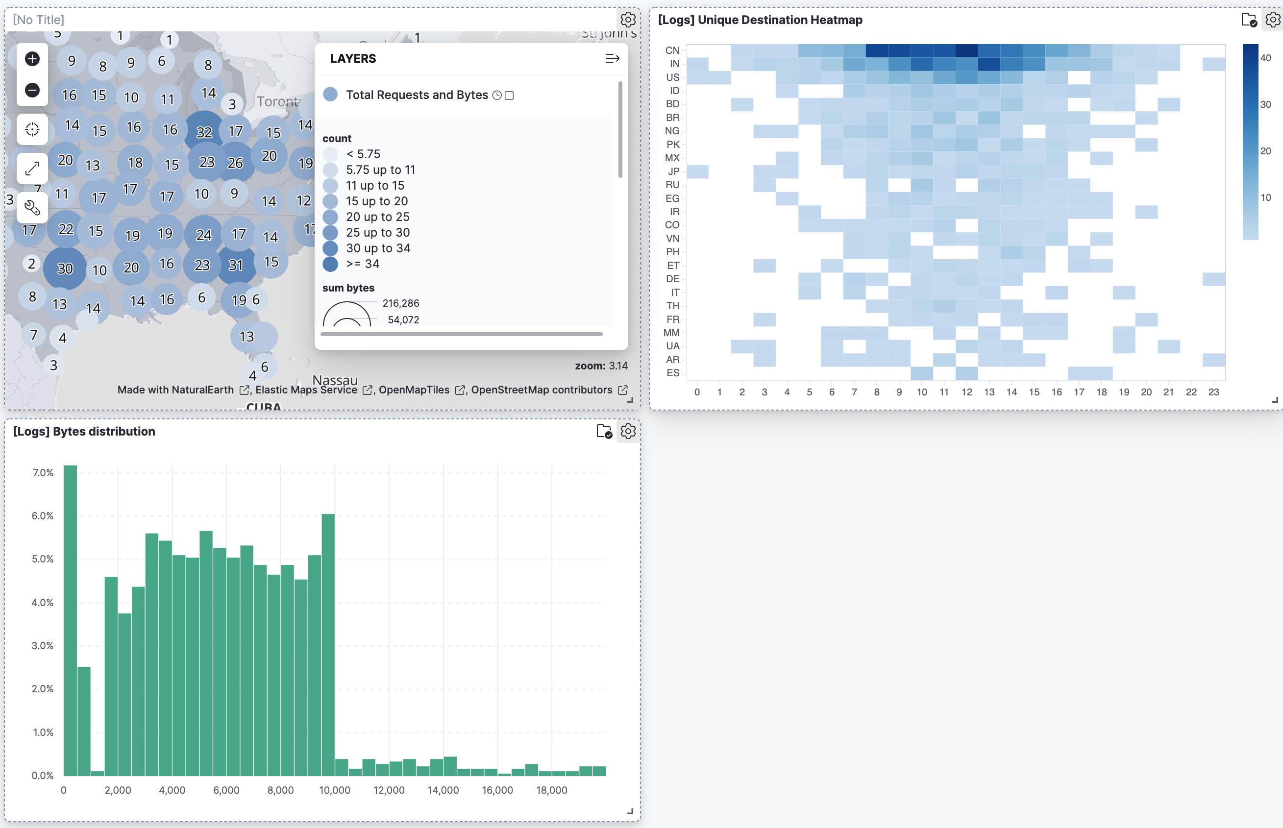
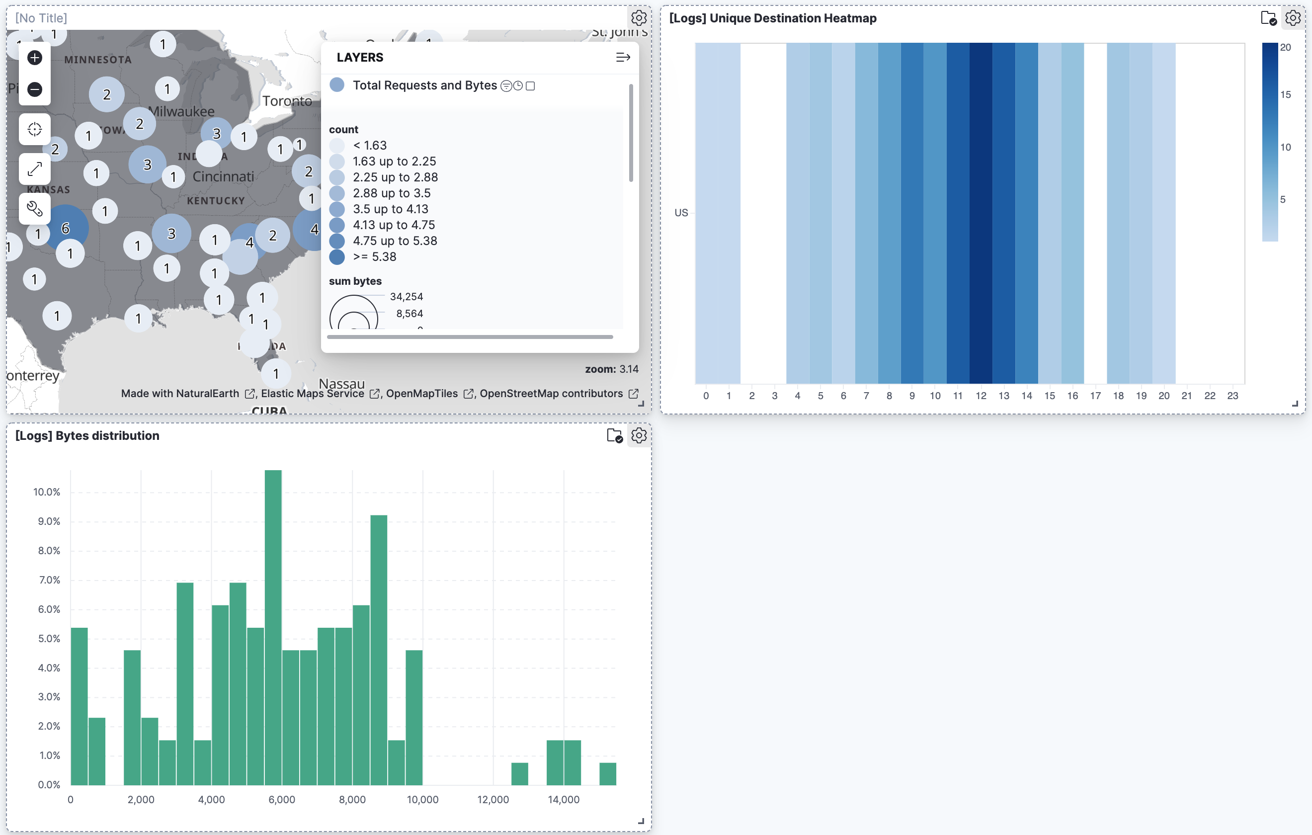
To filter for documents with unusually high byte values, select and drag across the high values in the Bytes distribution chart. The map and the heat map update.
To remove the filter, select the next to its name in the filter bar. All panels show the full data again.
Set a filter from the map:
Select anywhere on the United States to open a tooltip.
The tooltip has one page for each feature under your pointer. If it shows more than one page, use the arrows or the layer list to open the Total Requests by Destination page.
To keep only the requests whose destination is the United States, select Filter on property in the row for ISO 3166-1 alpha-2 code.
Kibana adds the filter
geo.dest: US, becausegeo.destis the field you joined in step 2.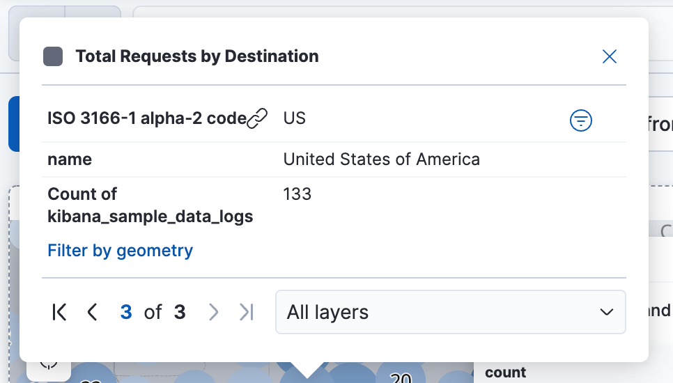
Your filtered dashboard should look similar to this:
The tooltip also has a Filter by geometry link, which filters by the country’s shape instead. Refer to Create a filter from a map.
You can interact with filter pills to edit them, temporarily alter their behavior without having to remove them, or make them available in other contexts. The following options are available when selecting a filter pill:
- Pin across all apps and Unpin
-
Adds this filter to available dashboards and to apps such as Discover, Lens, Maps, and Visualize. You remove the filter if you:
- Unpin it. In this case, the filter only remains on the currently open app, unpinned.
- Remove it from any place while it's still pinned.
- Refresh your session, for example by opening a dashboard in a new tab. Pinned filters are not saved along with the dashboard, visualization, or Discover session that you added them to.
TipWhen a pinned filter can't be applied, for example if a field specified in the filter doesn't exist in the current data view, the filter is ignored and shows in a different color.
- Edit filter
- Lets you edit and update the filter.
- Exclude results and Include results
- Reverses the filter behavior.
- Temporarily disable and Re-enable
- Lets you temporarily deactivate a filter instead of requiring you to remove it. This is particularly useful for testing different filter combinations.
- Delete
- Removes the filter.
You can perform most of these actions at once for all filters in your current view using the Query menu. From that menu, select Apply to all, then choose the action you'd like to perform.
- Check out additional types of layers that you can add to your map.
- Learn how terms joins match your data to boundaries.
- Learn more ways to customize your map.
- Learn more about vector tooltips.