Cost-saving strategies for the Elasticsearch Service: Data storage efficiency
Thousands of customers call the official Elasticsearch Service (ESS) on Elastic Cloud their home for running not only Elasticsearch, but exclusive products such as Elastic Logs, Elastic APM, Elastic SIEM, and more. With over seven years of operating experience, ESS is the only managed service that provides the complete Elasticsearch experience with all the features, all the solutions, and support from the source — as well as a number of operational and deployment benefits that complement these products.
In a previous post, we explained the hidden network cost of using a SaaS solution that’s not in the same region as your services, infrastructure, or logging devices, which can result in hefty fees. In this post, we’ll highlight how Elasticsearch Service on Elastic Cloud gives you the flexibility to choose various strategies to keep costs under control as your workloads expand.
With any growth, particularly in the observability and security spaces, the infrastructure required to store and analyze logs, metrics, APM traces, and security events generated by your applications increases, which brings additional costs. ESS offers a number of ways to help you manage your data to control costs while still retaining meaningful data for longer periods of time — and providing the same useful capabilities of the Elastic Stack: consolidation of data from various sources, visualization options, alerting, anomaly detection, and more.
We’ll review the cost-saving opportunities available for time-series data such as observability and security use cases. To illustrate, we’ll cover one of the most common applications that people use the Elastic Stack for: infrastructure monitoring. The Elastic Stack includes Beats, a collection of lightweight agents that live on your clients and ship data to your cluster. Metricbeat is widely used by teams to send system metrics like CPU usage, disk IOPS, or container telemetry for applications running on Kubernetes.
As you expand your application footprint, your monitoring needs will demand more storage to house the metrics being generated. Defining a retention period is one strategy that teams use today for managing time-series data at scale. We’ll explore additional storage efficiency options that are available right out of the box with ESS today.
Scenario
For continuity purposes, let’s dive into cost-saving strategies for a cluster that’s monitoring 1,000 hosts where each agent collects 100 bytes per metric and 100 metrics every 10 seconds, with a data retention period of 30 days. We’ll also store a replica of the data in the cluster for high availability, which prevents data loss in the event of a node failure. Let’s do the math to calculate how much storage we will require:
|
|
That puts our storage requirements at 5.2TB to store those metrics. For simplicity’s sake, we’ll ignore the storage demands that the Elasticsearch cluster requires for operation.
To summarize:
| Hosts monitored | 1,000 |
| Daily GB ingested | 86.4GB |
| Retention period | 30 days |
| Number of replicas | 1 |
| Storage requirements (including replicas) | 5.184TB |
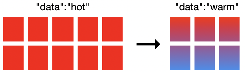
More efficient storage with hot-warm deployments and index lifecycle management
In observability use cases like logging and metrics, the utility of the data decreases over time. Typically teams leverage recent data to quickly investigate system incidents, sudden spikes in network traffic, or security alerts. As data ages, it becomes less frequently queried while still residing in the cluster and utilizing the same compute, memory, and storage resources as the rest of the cluster. This results in two very distinct data access patterns, but the cluster is only optimized for fast ingest and frequent querying, not for storage of infrequently accessed data.
Enter hot-warm architectures in Elasticsearch Service. This deployment option provides two hardware profiles in the same Elasticsearch cluster. Hot nodes handle all the fresh incoming data and have faster storage to ensure that they can ingest and retrieve data quickly. Warm nodes have a higher storage density and are more cost effective at storing data for longer retention periods.
In the Elasticsearch Service, we typically provision locally attached NVMe SSDs at a 1:30 RAM-to-disk ratio for hot nodes and highly dense HDDs at 1:160 for warm nodes. This powerful architecture goes hand in hand with another important feature: index lifecycle management (ILM). ILM provides the means to automate index management over time, which simplifies moving data from hot nodes to warm nodes based on certain criteria like index size, the number of documents, or the age of the index.
With these two features working together, you gain two distinct hardware profiles in your cluster — and the index automation tools to move the data between the tiers.
Now let’s migrate to a hot-warm deployment and configure ILM policies. In ESS, you can create a new hot-warm deployment and optionally restore a snapshot from another cluster. If you already have an existing high I/O deployment, you can simply migrate to a hot-warm deployment by adding warm nodes to your cluster. Using an ILM policy, we’ll keep data in the hot tier for seven days and then move the data to our warm nodes.
Under the hood, when data moves into the warm phase, indices can no longer be written to. This gives us another opportunity to save on costs as we can choose not to store any replica data in our warm nodes. In the event of a warm node failure, we would restore from the latest snapshot that was taken rather than from replicas.
The drawback with this approach is that restoring from a snapshot is typically slower and can increase your time to resolution after failure. However, in many cases this may be acceptable since warm nodes typically contain less frequently queried data, reducing real-world impact.
Finally, we’ll delete the data once it reaches 30 days of age to align with our original retention policy. Using similar math as we did above, here’s a summary of this approach:
| Traditional cluster | Hot-warm + ILM | |
| Hosts monitored | 1,000 | 1,000 |
| Daily GB ingested | 86.4GB | 86.4GB |
| Retention period | 30 days |
Hot: 7 days
Warm: 30 days |
| Replicas required | 1 |
Hot nodes: 1
Warm nodes: 0 |
| Storage requirements | 5.184TB |
Hot: 1.2096TB (w/ replicas)
Warm: 1.9872TB (no replicas) |
| Approximate cluster size required | 232GB RAM (6.8TB SSD storage) |
Hot: 58GB RAM with SSD
Warm: 15GB RAM with HDDs |
| Monthly cluster cost | $3,772.01 | $1,491.05 |
This approach saves a remarkable 60% in monthly costs while still having searchable and resilient data. You can fine-tune the ILM policies to find ideal rollover periods to help maximize the use of storage on warm nodes.
Free up more storage space with data rollups
Another storage saving option to consider is data rollups. By "rolling up" the data into a single summary document in Elasticsearch, the rollup APIs let you summarize the data and store it more compactly. You can then archive or delete the original data to gain storage space.
When you create a rollup, you get to pick all the fields you’re interested in for future analysis, and a new index is created with just that rolled-up data. This is especially helpful for monitoring use cases that primarily deal with numerical data that can easily be summarized at a higher granularity such as at a minute, hourly, or even daily level while still continuing to show trends over time. Summarized indices are available throughout Kibana and can easily be added alongside existing dashboards to avoid disruptions in any analysis efforts. This can all be configured directly in Kibana.
Continuing with the scenario above, recall that we required 5.2TB of storage space to store 30 days’ worth of metrics data from 1,000 hosts, including a replica set to ensure high availability. We then described a scenario using a hot-warm deployment template. Now we’ll use the data rollups API to configure a rollup job to execute when data is seven days old and sacrifice a little less granularity while gaining much more free storage.
Let’s set the data rollup job to roll up our 10-second metrics data into hourly summarized documents. This will still let us query and visualize our older metrics at hourly intervals, which can be used in Kibana visualizations and Lens to reveal trends and other key moments in the data. Next we’ll delete the original documents that we just rolled up, freeing a large amount of storage in the cluster. If we do the math, we can calculate how storage is required for the data we just rolled up.
|
|
The original data of these rolled-up documents was older than seven days and therefore stored in warm nodes in our hot-warm cluster. All of that 1.99TB of data can simply be deleted. The column on right showcases where we just ended up:
| Traditional cluster | Hot-warm + ILM | Hot-warm + ILM with rolled-up data | |
| Hosts monitored | 1,000 | 1,000 | 1,000 |
| Daily GB ingested | 86.4GB | 86.4GB | 86.4GB |
| Retention period | 30 days |
Hot: 7 days
Warm: 30 days |
Hot: 7 days
Warm: 30 days |
| Granularity | 10 seconds | 10 seconds |
First 7 days: 10 seconds
After 7 days: 1 hour |
| Replicas required | 1 |
Hot nodes: 1
Warm nodes: 0 |
Hot nodes: 1
Warm nodes: 0 |
| Storage requirements | 5.184TB |
Hot: 1.2096TB (w/ replicas)
Warm: 1.9872TB (no replicas) |
Hot: 1.2096TB (w/ replicas)
Warm: 5.52GB (no replicas, rolled-up data) |
| Approximate cluster size required | 232GB RAM (6.8TB SSD storage) |
Hot: 58GB RAM with SSDs
Warm: 15GB RAM with HDDs |
Hot: 58GB RAM with SSDs
Warm: 2GB RAM with HDDs |
| Monthly cluster cost | $3,772.01 | $1,491.05 | $1,024.92 |
The difference in cost savings is dramatic. When we add data rollups to our existing hot-warm cluster, we can attain a 31% reduction in costs. The results are even more amplified when we compare our final scenario to a traditional single hardware tier cluster and save 73%!
Deploy your own way
Each method has its own benefits and tradeoffs. You have the flexibility to fine-tune each strategy to best fit your needs.
ILM policies let you define rollover periods based on index size, the number of documents, or document age, which moves data into warm nodes in your hot-warm cluster. Warm nodes can pack a lot of storage efficiently, helping you spend less on compute costs. Query times may not be as performant as hot nodes, making this a preferred approach for data that’s infrequently queried.
Data rollups summarize data into less granular documents, which proves useful if the data has aged to a point where the original low-level granularity is no longer required. The source documents can then be deleted helping you save on storage costs. You can define how high to summarize documents up to, and also when. Find the right balance so that your rolled-up data continues to provide you with key insights such as trends over time or system behavior from a traffic spike.
Now that you’re familiar with out-of-the-box strategies for optimizing metrics workloads in your Elasticsearch cluster, what should you do with all that extra storage space? The Elastic Stack is used all over the world for a myriad of use cases: logs, APM traces, audit events, endpoint data, and more.
Elasticsearch Service on Elastic Cloud provides everything the Elastic Stack has to offer coupled with operational expertise from the creators. If you’re not ready to expand into new use cases, you can continue putting your cluster to work by leveraging storage optimization. Expand your data retention time and store even more at a similar price point, or reduce your cluster size with a few clicks without having to compromise on visibility — and save.
Looking to get started with the Elasticsearch Service on Elastic Cloud? Spin up a free 14-day trial.