Add flexibility to your data science with inference pipeline aggregations
Elastic 7.6 introduced the inference processor for performing inference on documents as they are ingested through an ingest pipeline. Ingest pipelines are incredibly powerful and flexible but they are designed to work at ingest. So what happens if your data is already ingested?
Introducing the new Elasticsearch inference pipeline aggregation, which lets you apply new inference models on data that's already been indexed. With this new aggregation type, you can use the machine learning inference at search in an aggregation and get the results instantly — in real time with the latest data. Now you can always look forward to new models without worrying about reindexing your data in Elasticsearch!
This blog will show you how to use the inference pipeline aggregation to apply a new model to existing data (for our example, we'll use customer service churn data), and will then show you how to dashboard the inference results with the Kibana Vega plugin. If you'd like to try it yourself, you can spin up a free trial of Elastic Cloud or enable a free trial of machine learning on a local install.
Inference pipeline aggregations
Inference is the process of making predictions against a model trained by machine learning algorithms. The Elastic Stack supports two types of models: regression models, which are trained to find relationships in the data and predict a numerical value such as house price, and classification models, which predict which category or class the data point falls into.
The input to a model can be numerical values, categorical (text/keyword field), or even IP addresses. A pipeline aggregation is an aggregation that takes the output of other aggregations as its input. These might be numerical values, keywords, or even IP addresses — and now you can see the start of a beautiful friendship.
Example: Applying a new customer churn model
The data set we'll be using was first presented in the Introduction to supervised machine learning in Elastic webinar. In that webinar, we used fictional telecom call record data (from OpenML and Kaggle) to predict which customers will churn given their history. A subset of the customer records have been marked up with a target churn field, making them suitable for training a model with supervised learning. Experimentation has shown features such as the total call charges and the number of customer service calls are particularly significant predictors of churn.
We have the trained model from the webinar that tells us which customers are at risk of churning — now it is time to use it. In this blog, I'm going to show you how to execute that same model at search (not ingest) so you can view the inference predictions instantly on the latest data.
Top Tip: When sharing a model between clusters, use the for_export parameter in the Get trained model request to return the model in a format that can be directly uploaded to a different cluster.
Step 1: Ingest customer churn data
Download the data set and install the trained model to get started with this example:
- Download calls.csv and customers.csv.
- Import the CSVs using the Data Visualizer in Kibana, creating the calls and customer indices. If you don't have a Kibana instance handy, spin up a free trial of Elastic Cloud.
- Download telco_churn_model.json.
- Upload the churn model to your cluster with this curl command, changing user:password and localhost:9200 as appropriate.
curl -u user:password -XPUT -H "Content-Type: application/json" "http://localhost:9200/_ml/inference/telco_churn" -d @telco_churn_model.json
Step 2: Using the inference aggregation
The customer call data you just ingested is normalized and split across two indices — customers and calls. Phone numbers are unique to customers and occur in both indices; a composite terms aggregation on the phone_number field is used to create the customer entity and the features are constructed via subaggregations. The inference aggregation is a parent pipeline aggregation that operates on each bucket or entity.
Run the inference aggregation below from within the Console:
GET calls,customers/_search
{
  "size": 0,
  "aggs": {
    "phone_number": {
      "composite": {
        "size": 100,
        "sources": [
          {
            "phone_number": {
              "terms": {
                "field": "phone_number"
              }
            }
          }
        ]
      },
      "aggs": {
        "call_charges": {
          "sum": {
            "field": "call_charges"
          }
        },
        "call_duration": {
          "sum": {
            "field": "call_duration"
          }
        },
        "call_count": {
          "value_count": {
            "field": "dialled_number"
          }
        },
        "customer_service_calls": {
          "sum": {
            "field": "customer_service_calls"
          }
        },
        "number_vmail_messages": {
          "sum": {
            "field": "number_vmail_messages"
          }
        },
        "account_length": {
          "scripted_metric": {
            "init_script": "state.account_length = 0",
            "map_script": "state.account_length = params._source.account_length",
            "combine_script": "return state.account_length",
            "reduce_script": "for (d in states) if (d != null) return d"
          }
        },
        "international_plan": {
          "scripted_metric": {
            "init_script": "state.international_plan = ''",
            "map_script": "state.international_plan = params._source.international_plan",
            "combine_script": "return state.international_plan",
            "reduce_script": "for (d in states) if (d != null) return d"
          }
        },
        "voice_mail_plan": {
          "scripted_metric": {
            "init_script": "state.voice_mail_plan = ''",
            "map_script": "state.voice_mail_plan = params._source.voice_mail_plan",
            "combine_script": "return state.voice_mail_plan",
            "reduce_script": "for (d in states) if (d != null) return d"
          }
        },
        "state": {
          "scripted_metric": {
            "init_script": "state.state = ''",
            "map_script": "state.state = params._source.state",
            "combine_script": "return state.state",
            "reduce_script": "for (d in states) if (d != null) return d"
          }
        },
        "churn_classification": {
          "inference": {
            "model_id": "telco_churn",
            "inference_config": {
              "classification": {
                "prediction_field_type": "number"
              }
            },
            "buckets_path": {
              "account_length": "account_length.value",
              "call_charges": "call_charges.value",
              "call_count": "call_count.value",
              "call_duration": "call_duration.value",
              "customer_service_calls": "customer_service_calls.value",
              "international_plan": "international_plan.value",
              "number_vmail_messages": "number_vmail_messages.value",
              "state": "state.value"
            }
          }
        }
      }
    }
  }
}
Granted, this looks complicated because each feature expected by the model is computed with a subaggregation. But let’s focus on the inference configuration, which is relatively simple.
"inference": {
  "model_id": "telco_churn",
  "inference_config": {
    "classification": {
      "prediction_field_type": "number"
    }
  },
  "buckets_path": {
    "account_length": "account_length.value",
    "call_charges": "call_charges.value",
    "call_count": "call_count.value",
    "call_duration": "call_duration.value",
    "customer_service_calls": "customer_service_calls.value",
    "international_plan": "international_plan.value",
    "number_vmail_messages": "number_vmail_messages.value",
    "state": "state.value"
  }
}
The required fields are model_id — in this case the id of the previously trained model I was given — and buckets_path, a map detailing the inputs using the standard pipeline aggs bucket path syntax. The inference_config section specifies that the output should be a number rather than a string, which will prove useful in a moment.
The output of the inference aggregation with the other aggs elided looks like this:
"aggregations" : {
  "phone_number" : {
    "meta" : { },
    "after_key" : {
      "phone_number" : "408-337-7163"
    },
    "buckets" : [
      {
        "key" : {
          "phone_number" : "408-327-6764"
        },
        ...
        "churn_classification" : {
          "value" : 0,
          "prediction_probability" : 0.9748441804026897,
          "prediction_score" : 0.533111462991059
        }
      },
      ...
    }
  }
}
value: 0 indicates the customer will not churn and the prediction probability tells us the model is confident of the result.
We can see the predictions but the customers we are really interested in are those who the model predicts will churn. To find those fickle users we can filter with a bucket_selector aggregation:
"will_churn_filter": {
  "bucket_selector": {
    "buckets_path": {
      "will_churn": "churn_classification>value"
    },
    "script": "params.will_churn > 0"
  }
}
And now we only see the churners. The script requires the output of the aggregation is a numerical value, which is why we set "prediction_field_type": "number" in the inference configuration.
Step 3: Visualizing the results in Kibana
This is great, but the results format is a lot to parse if you’re not a computer! How can I get a quick overview such as a count of those who will churn against those who will not? Preferably a visual one? Stand up the versatile Kibana Vega plugin, which can both transform data and visualize it.
The data source is the same query as above and a Vega transform is used to group the classification results by predicted class and produce a count of each type. First, a lookup is used to give meaningful names to the numerical predicted class value.
"transform": [
  {
    "lookup": "churn_classification.value",
    "from": {
      "data": {
        "values": [
          {"category": 0, "classification_class": "Won't Churn"},
          {"category": 1, "classification_class": "Will Churn"}
        ]
      },
      "key": "category",
      "fields": ["classification_class"]
    }
  },
  {
    "aggregate": [
      {
        "op": "count",
        "as": "class_count"
      }
    ],
    "groupby": ["classification_class"]
  }
],
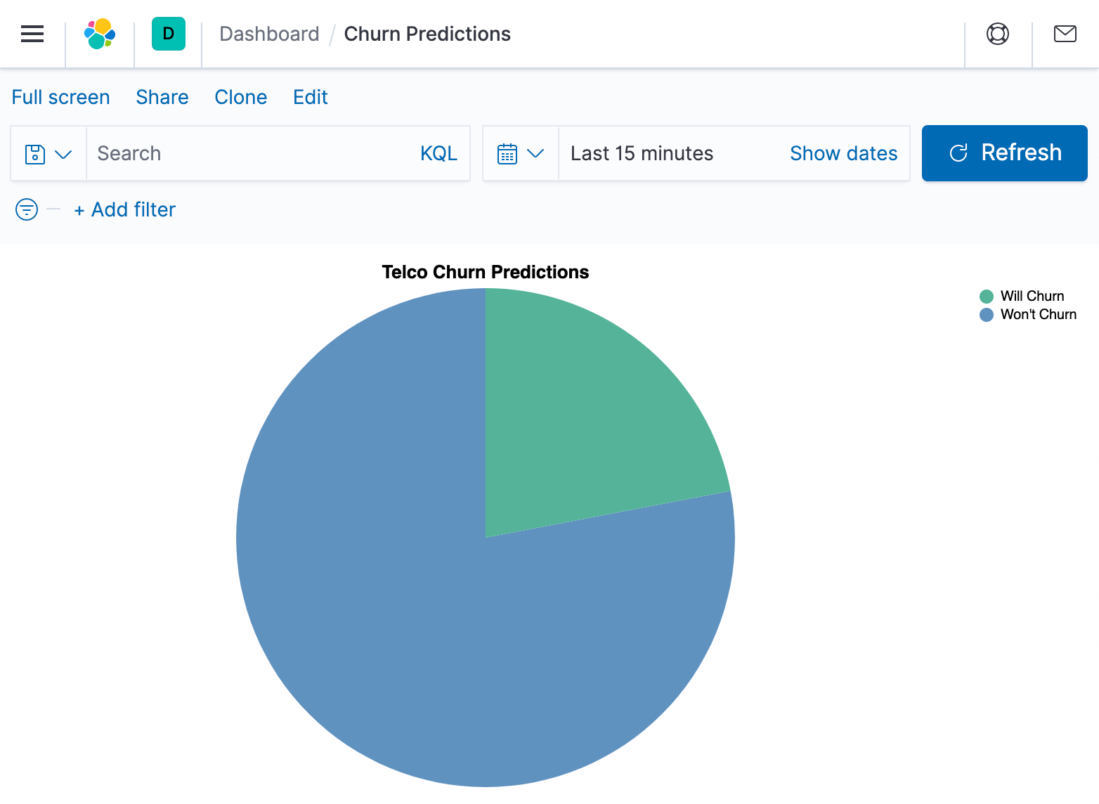
Then draw a pie chart of the inference results.
"mark": "arc",
"encoding": {
  "theta": {"field": "class_count", "type": "quantitative"},
  "color": {"field": "classification_class", "type": "nominal", "legend": {"title": null }}
}
And we can save this as a simple dashboard.
All the search and vega configurations are stored in the Gist for this blog.
Conclusion
Everybody wants to use their historical data to make better business decisions, and this is a very practical, straightforward way to do just that. By using a machine learning model, the inference aggregation can quickly and easily be utilized to find customers on the verge of churning. Make predictions in real time and use the Kibana Vega visualization to dashboard the results.
It is simple to get started — train a model using Elastic’s data frame analytics or import an existing one with the Eland Python client. Try it for yourself today with a free trial of Elastic Cloud.