Sizing Hot-Warm Architectures for Logging and Metrics in the Elasticsearch Service on Elastic Cloud
Want to learn more about the differences between the Amazon Elasticsearch Service and our official Elasticsearch Service? Visit our AWS Elasticsearch comparison page.
These are exciting times! Elasticsearch Service on Elastic Cloud recently added support for a wide range of hardware choices and deployment templates, which makes it perfectly suited for efficient handling of logging and metrics related workloads. With all this new flexibility comes a lot of choices to be made. Picking the most appropriate architecture for your use-case and estimating the required cluster size can be tricky. Don’t worry — we are here to help!
This blog post will teach you about the different architectures that are commonly used for logging and metrics use cases and when to use them. It will also provide guidance on how to size and manage your cluster(s) so you get the most out of them.
What architectures are available for my logging cluster?
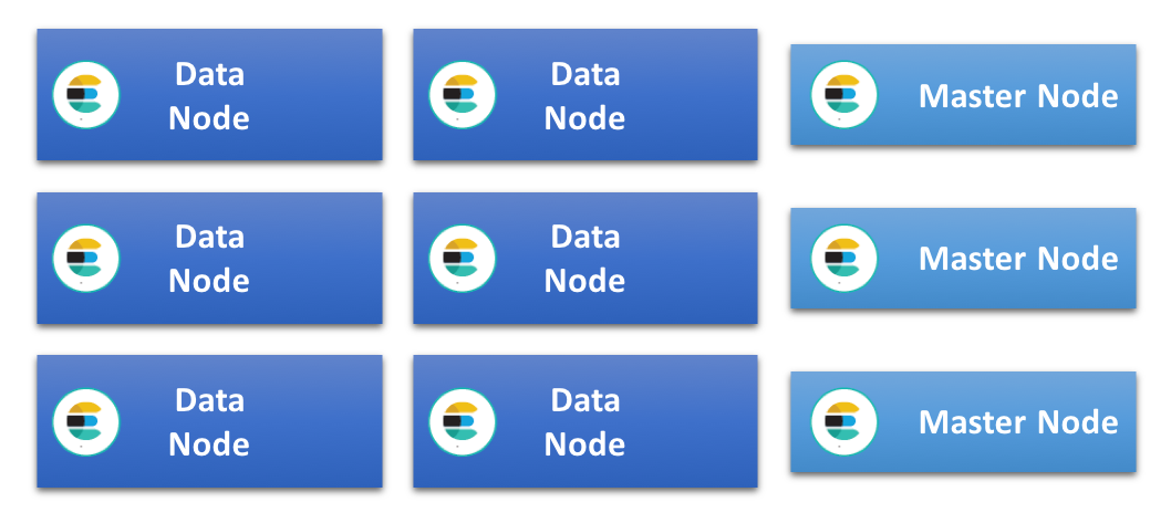
In the simplest of all Elasticsearch clusters, all data nodes have the same specification and handle all roles. As this type of cluster grows, nodes for specific tasks are often added, e.g. dedicated master, ingest and machine learning nodes. This takes load off the data nodes and allows them to operate more efficiently. In this type of cluster all data nodes share the indexing and query load evenly, and as they all have the same specification, we often refer to this as a homogenous or uniform cluster architecture.
Another architecture that is very popular, especially when working with time-based data like logs and metrics, is what we refer to as the hot-warm architecture. This relies on the principle that data generally is immutable and can be indexed into time-based indices. Each index thus contains data covering a specific time period, which makes it possible to manage retention and life cycle of data by deleting full indices. This architecture has two different types of data nodes with different hardware profiles: ‘hot’ and ‘warm’ data nodes.
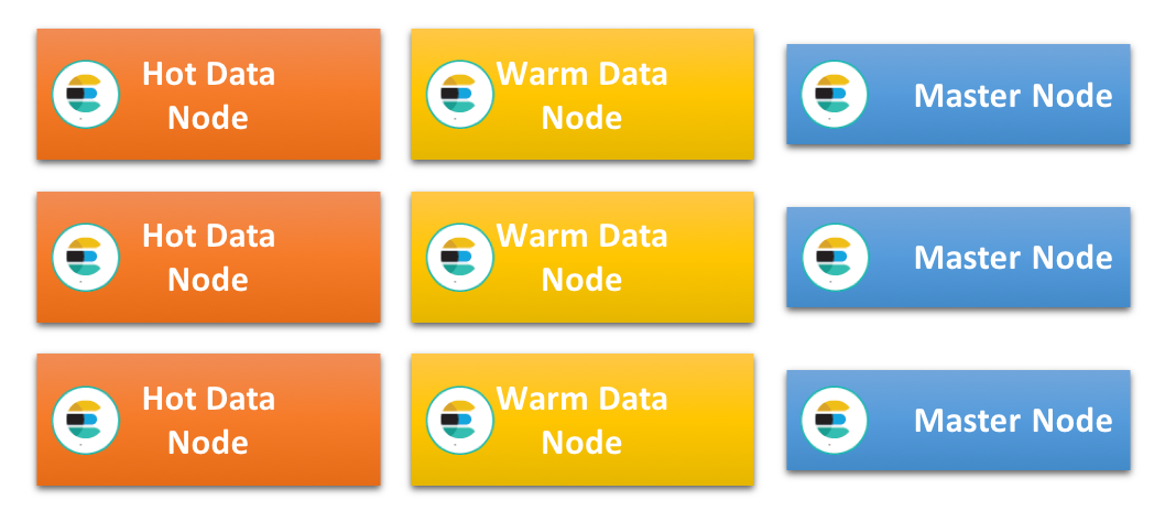
Hot data nodes hold all the most recent indices and therefore handle all indexing load in the cluster. As the most recent data also typically is the most frequently queried, these nodes tend to get very busy. Indexing into Elasticsearch can be very CPU and I/O intensive, and the additional query load means that these nodes need to be powerful and have very fast storage. This generally means local, attached SSDs.
Warm nodes on the other hand are optimized to handle long-term storage of read-only indices in the cluster in a cost efficient way. They are generally equipped with good amounts of RAM and CPU but often uses local attached spinning disks or SAN instead of SSDs. Once indices on the hot nodes exceed the retention period for those nodes and are no longer indexed into, they get relocated to the warm nodes.
It is important to note that moving data from hot to warm nodes does not necessarily mean that it will be slower to query. As these nodes do not handle any resource intensive indexing at all, they are often able to efficiently serve queries against older data at low latencies without having to utilize SSD based storage.
As data nodes in this architecture are very specialized and can be under high load, it is recommended to use dedicated master, ingest, machine learning and coordinating-only nodes.
Which architecture should I pick?
For a lot of use-cases either of these architectures will work well, and which one to pick is not always clear. There are however certain conditions and constraints that may make one of the architectures more suitable than the other.
The type(s) of storage available to the cluster is an important factor to consider. As a hot/warm architecture requires very fast storage for the hot nodes, this architecture is not suitable if the cluster is limited to the use of slower storage. In this case it is better to use a uniform architecture and spread out indexing and querying across as many nodes as possible.
Uniform clusters are often supported by local spinning disks or SAN attached as block storage, even though SSDs are getting more and more common. Slower storage may not be able to support very high indexing rates, especially when there is also concurrent querying, so it can take a long time to fill up the available disk space. Holding large data volumes per node may therefore only be possible if you have a reasonably long retention period.
If the use-case stipulates a very short retention period, e.g. less than 10 days, data will not sit idle on disk for long once indexed. This requires performant storage. A hot/warm architecture may work, but a uniform cluster with just hot data nodes may be better and easier to manage.
How much storage do I need?
One of the main drivers when sizing a cluster for a logging and/or metrics use case is the amount of storage. The ratio between the volume of raw data and how much space this will take up on disk once indexed and replicated in Elasticsearch will depend a lot on the type of data and how this is indexed. The diagram below shows the different stages the data goes through during indexing.
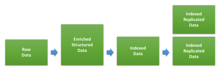
The first step involves transforming the raw data into the JSON documents we will index into Elasticsearch. How much this changes the size of the data will depend on the original format and the structure added, but also the amount of data added through various types of enrichment. This can differ significantly for different types of data. If your logs are already in JSON format and you are not adding any additional data, the size may not change at all. If you on the other hand have text based web access logs, the added structure and information about user agent and location might be considerably larger.
Once we index this data into Elasticsearch, the index settings and mappings used will determine how much space it takes up on disk. The default dynamic mappings applied by Elasticsearch are generally designed for flexibility rather than optimized storage size on disk, so you can save disk space by optimizing the mappings you use through custom index templates. Further guidance around this can be found in the tuning documentation.
In order to estimate how much disk space a specific type of data will take up in your cluster, index a large enough amount of data to make sure you reach the shard size you are likely to use in production. Testing using too small data volumes is a quite common mistake that can give inaccurate results.
How do I balance ingest and querying?
The first benchmark most users run when sizing a cluster is often to determine the maximum indexing throughput of the cluster. This is, after all, a benchmark that is quite easy to set up and run, and the results can also be used to determine how much space the data will take up on disk.
Once the cluster and ingest process has been tuned and we have identified the maximum indexing rate we can sustain, we can calculate how long it would take to fill up the disk on the data nodes if we could keep indexing at maximum throughput. This will give us an indication of what the minimum retention period would be for the node type assuming we want to maximize the use of the available disk space.
It may be tempting to directly use this to determine the size needed, but that would not leave any headroom for querying, as all system resources would be used for indexing. After all, most users are storing the data in Elasticsearch in order to be able to query it at some point and expect good performance when doing so.
How much headroom do we then need to leave for querying? This is a difficult question to give a generic answer to as it depends a lot on the amount and nature of querying that is expected as well as what latencies users expect. The best way to determine this is to run a benchmark simulating realistic levels of querying at different data volumes and indexing rates as described in this Elastic{ON} talk about quantitative cluster sizing and this webinar about cluster benchmarking and sizing using Rally.
Once we have determined how large a portion of the maximum indexing throughput we can sustain while at the same time serve queries to users with acceptable performance, we can adjust the expected retention period to match this reduced indexing rate. If we index at a slower pace, it will take longer to fill up the disks.
This adjustment may give us the ability to handle small peaks in traffic, but generally assumes a quite constant indexing rate over time. If we expect our traffic levels to have peaks and fluctuate throughout the day, we may need to assume the adjusted indexing rate corresponds to to the peak level and even further reduce the average indexing rate we assume each node can handle. In the case where fluctuations are predictable and last for extended periods of time, e.g. during office hours, another option may be to increase the size of the hot zone just for that period.
How do I use all this storage?
In hot-warm architectures, the warm nodes are expected to be able to hold large amounts of data. This also applies to data nodes in a uniform architecture with a long retention period.
Exactly how much data you can successfully hold on a node often depends on how well you can manage heap usage, which often becomes the main limiting factor for dense nodes. As there are a number of areas that contribute to heap usage in an Elasticsearch cluster — e.g. indexing, querying, caching, cluster state, field data and shard overhead — the results will vary between use-cases. The best way to accurately determining what the limits are for your use-case is to run benchmarks based on realistic data and query patterns. There are however a number of generic best practices around logging and metrics use-cases that will help you get as much from your data nodes as possible.
Make sure mappings are optimized
As described earlier, the mappings used for your data can affect how compact it is on disk. It can also affect how much field data you will use and impact heap usage. If you are using Filebeat modules or Logstash modules to parse and ingest your data, these come with optimized mappings out of the box, and you may not need to worry too much about this point. If you however are parsing custom logs and are relying extensively on the ability of Elasticsearch to dynamically map new fields, you should continue reading.
When Elasticsearch dynamically maps a string, the default behaviour is to use multi-fields to map the data both as text, which can be used for case-insensitive free-text search, and keyword, which is used when aggregating data in Kibana. This is a great default as it gives optimal flexibility, but the downside is that it increases the size of indices on disk and the amount of field-data used. It is therefore recommended to go through and optimize mappings wherever possible, as this can make a significant difference as data volumes grow.
Keep shards as large as possible
Each index in Elasticsearch contains one or more shards, and each shard comes with overhead that uses some heap space. As described in this blog post about sharding, smaller shards have more overhead per data volume compared to larger shards. In order to minimize heap usage on nodes that are to hold large amounts of data, it is therefore important to try to keep shards as large as possible. A good rule of thumb is to keep the average shard size for long-term retention at between 20GB and 50GB.
As each query or aggregation runs single-threaded per shard, the minimum query latency will typically depend on the shard size. This depends on data and queries, so can vary even between indices within the same use-case. For a specific data volume and type of data, it is, however, not certain that a larger number of smaller shards will perform better than a single larger shard.
It is important to test the effect of shards size in order to reach an optimum with respect to query usage and minimal overhead.
Tune for storage volume
Efficiently compressing the JSON source can have a significant impact on how much space your data takes up on disk. Elasticsearch by default compresses this data using a compression algorithm tuned for balance between storage and indexing speed, but also offers a more aggressive one as an option – the best_compression codec.
This can be specified for all new indices but comes with a performance penalty of around 5-10% during indexing. The disk space gain can be significant, so it may be a worthwhile trade-off.
If you have followed the advice in the previous section and are force merging indices, you also have the option to apply the improved compression just before the force merge operation.
Avoid unnecessary load
The last thing contributing to heap usage that we are going to discuss here is request handling. All requests that are sent to Elasticsearch are coordinated at the node they arrive. The work is then partitioned and spread out to where the data resides. This applies to indexing as well as querying.
Parsing and coordinating the request and response can result in significant heap usage. Make sure that nodes working as coordinating or indexing nodes have enough heap headroom to be able to handle this.
For nodes tuned for long-term data storage, it often makes sense to let them work as dedicated data nodes and minimize any additional work they need to perform. Directing all queries either to hot nodes or dedicated coordinating only nodes can help achieve this.
How do I apply this to my Elasticsearch Service deployment?
The Elasticsearch Service is currently available on AWS and GCP, and although the same instance configurations and deployment templates are available on both platforms, the specification differs a little. In this section we will look at the different instance configurations and how these fit in with the architectures we discussed earlier. We will also look at how we can go about estimating the size of the cluster needed to support an example use-case.
Editor’s Note (September 3, 2019): Microsoft Azure is now available as a cloud provider for Elasticsearch Service on Elastic Cloud. For more information, please read the announcement blog.
Available instance configurations
The Elasticsearch Service has traditionally had Elasticsearch nodes backed by fast SSD storage. These are referred to as highio nodes, and have excellent I/O performance. This makes them very well suited as hot nodes in a hot-warm architecture, but they can also be used as data nodes in a Uniform architecture. This is often recommended if you have a short retention period that requires performant storage.
On AWS and GCP highio nodes have a disk to RAM ratio of 30:1, so for every 1 GB of RAM there is 30GB of storage available. Available node sizes on AWS are 1GB, 2GB, 4GB, 8GB, 15GB, 29GB and 58GB, while the GCP nodes come in the sizes 1GB, 2GB, 4GB, 8GB, 16GB , 32GB and 64GB.
Another node type that has recently been introduced on Elastic Cloud is the storage optimized highstorage node. These are equipped with large volumes of slower storage, and have a 100:1 disk to RAM ratio. A 64GB highstorage node on GCP comes with over 6.2TB of storage while a 58GB node on AWS supports 5.6TB. These node types come in the same RAM sizes as highio nodes on the respective platform.
These nodes are typically used as warm nodes in a hot/warm architecture. Benchmarks on highstorage nodes have shown that this type of node on GCP have a significant performance advantage compared to AWS, even after the difference in size has been accounted for.
Using 2 or 3 availability zones
In most regions, you have an option to choose running on either 2 or 3 availability zones, and you can choose a different number of nodes per zone in the cluster. When staying within a fixed number of availability zones, the available cluster sizes increase by roughly doubling in size, at least for smaller clusters. If you are open to using either 2 or 3 availability zones, you can size in smaller steps, as going from 2 to 3 availability zones with the same node size increases capacity by only 50%.
Sizing example: Hot-warm architecture
In this example, we will look at sizing a hot-warm cluster that is able to handle ingestion of 100GB of raw web access logs per day with a retention period of 30 days. We will compare deploying this with Elastic Cloud on AWS and GCP.
Please note that the data used here are just an example, and it is very likely that your use-case will be different.
Step1: Estimate total data volume
For this example, we are assuming that the data is ingested using Filebeat modules and that the mappings therefore are optimized. We are sticking to a single type of data for simplicity in this example. During indexing benchmarks, we have seen that the ratio between the size of raw data and the indexed size on disk is around 1.1, so 100GB of raw data is estimated to result in 110GB of indexed data on disk. Once a replica has been added that doubles to 220GB.
Over 30 days that gives a total indexed and replicated data volume of 6600GB that the cluster as a whole need to handle.
This example assumes 1 replica shard is used across all zones, as this is considered best practice for performance and availability.
Step 2: Size hot nodes
We have run some maximum indexing benchmarks against hot nodes using this data set, and we have seen that it takes around 3.5 days for disks on highio nodes to fill up on AWS and GCP.
In order to leave some headroom for querying and small peaks in traffic, we will assume we can only sustain indexing at no more than 50% of the maximum level. If we want to be able to fully utilize the storage available on these nodes we therefore need to index into the node during a longer time period, and we therefore adjust the retention period on these nodes to reflect that.
Elasticsearch also needs some spare disk space to work efficiently, so in order to not exceed the disk watermarks we will assume a cushion of 15% extra disk space is required. This is shown in the Disk space needed column below. Based on this, we can determine the total amount of RAM needed for each provider.
| Platform | Disk:RAM Ratio | Days to Fill | Effective Retention (days) | Data Volume Held (GB) | Disk Space Needed (GB) | RAM Required (GB) | Zone Specification |
| AWS | 30:1 | 3.5 | 7 | 1440 | 1656 | 56 | 29GB, 2AZ |
| GCP | 30:1 | 3.5 | 7 | 1440 | 1656 | 56 | 32GB, 2AZ |
Step 3: Size warm nodes
The data that exceeds the retention period on the hot nodes will be relocated to the warm nodes. We can estimate the size needed by calculating the amount of data these nodes need to hold, taking the overhead for high watermarks into account.
| Platform | Disk:RAM Ratio | Effective Retention (days) | Data Volume Held (GB) | Disk Space Needed (GB) | RAM Required (GB) | Zone Specification |
| AWS | 100:1 | 23 | 5060 | 5819 | 58 | 29GB, 2AZ |
| GCP | 100:1 | 23 | 5060 | 5819 | 58 | 32GB, 2AZ |
Step 4: Add additional node types
In addition to the data nodes, we generally also need 3 dedicated master nodes in order to make the cluster more resilient and highly available. As these do not serve any traffic, they can be quite small. Initially allocating 1GB to 2GB nodes across 3 availability zones is a good size to start with. Then scale these nodes up to about 16GB across 3 availability zones as the size of the managed cluster grows.
What’s next?
If you haven’t already, start your 14-day free trial of the Elasticsearch Service and try this out! See for yourself how easy it is to set up and manage. If you have any questions, or want additional advice on how to size your Elasticsearch Service on Elastic Cloud, either contact us directly or engage with us through our public Discuss forum.