Analyze and visualize Strava activity details with the Elastic Stack


 Share on Twitter
Share on Twitter

 Share on LinkedIn
Share on LinkedIn

 Share on Facebook
Share on Facebook

 Share by Email
Share by Email

 Print this page
Print
This is the second blog post in our Strava series, based on the first one: “How to import Strava data into the Elastic Stack.” I will take you through a journey of data onboarding, manipulation, and visualization.
What is Strava and why is it the focus? Strava is a platform where athletes, from recreational to professional, can share their activities. All my fitness data from my Apple Watch, Garmin, and Zwift is automatically synced and saved there. It is safe to say that if I want to get an overview of my fitness, getting the data out of Strava is the first step.
Why do this with the Elastic Stack? I want to ask my data questions, and questions are just searches!
- Have I ridden my bike more this year than last?
- On average, is my heart rate reduced by doing more distance on my bike?
- Am I running, hiking, and cycling on the same tracks often?
- Does my heart rate correlate with my speed when cycling?
Detailed data analysis
In the last blog, we captured that Strava provides a general activity overview that gives you the total distance, average speed, and average heart rate. Since we want to take control of our data and do an in-depth analysis, we need more granular data. Strava has an API called streams, and a stream represents a single type of metric: time, distance, heart rate, cadence, gradient, etc.
The activity in Strava has a duration of 1 hour, 14 minutes, and 8 seconds. It is a virtual cycling activity, where I rode the Cobbled Climbs in Richmond, Virginia.
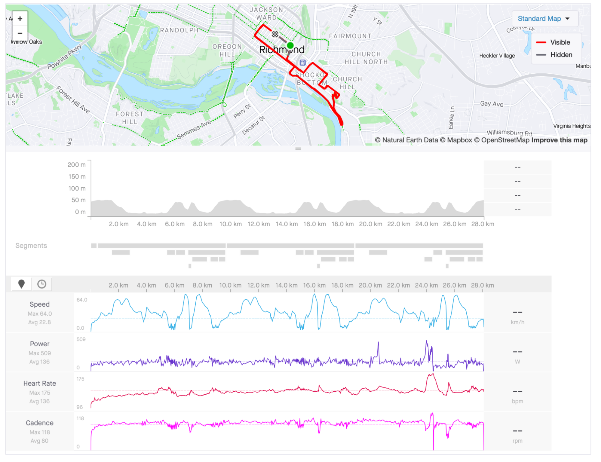
We need to run the streams API call using an activity id. This answer can contain multiple streams, as explained above. We will look at the document when we collect all available streams.
{
   "watts": {
       "data": [
           86,
           62,
           58,
           38,
           53,
           63,
           30,
           ...
       ],
       "series_type": "distance",
       "original_size": 4444,
       "resolution": "high"
   },
   "moving": {
       "data": [
           false,
           true,
           true,
           ...
       ],
       "series_type": "distance",
       "original_size": 4444,
       "resolution": "high"
   },
   "latlng": {
       "data": [
           [
               37.539652,
               -77.431735
           ],
           [
               37.53966,
               -77.43175
           ],
           [
               37.539667,
               -77.431768
           ],
           [
               37.539676,
               -77.431785
           ],
           [
               37.539684,
               -77.431802
           ],
           ...
       ],
       "series_type": "distance",
       "original_size": 4444,
       "resolution": "high"
   },
   "velocity_smooth": {
       "data": [
           0.0,
           1.59,
           1.665,
           1.693,
           1.723,
           1.73,
           ...
       ],
       "series_type": "distance",
       "original_size": 4444,
       "resolution": "high"
   },
   "grade_smooth": {
       "data": [
           0.0,
           2.9,
           2.3,
           3.7,
           2.0,
           ...
       ],
       "series_type": "distance",
       "original_size": 4444,
       "resolution": "high"
   },
   "cadence": {
       "data": [
           21,
           26,
           27,
           27,
           27,
           28,
           29,
           50,
           4,
           ...
       ],
       "series_type": "distance",
       "original_size": 4444,
       "resolution": "high"
   },
   "distance": {
       "data": [
           1.9,
           3.5,
           5.3,
           7.0,
           8.8,
           ...
       ],
       "series_type": "distance",
       "original_size": 4444,
       "resolution": "high"
   },
   "altitude": {
       "data": [
           48.4,
           48.4,
           50.1,
           ...
       ],
       "series_type": "distance",
       "original_size": 4444,
       "resolution": "high"
   },
   "heartrate": {
       "data": [
           104,
           104,
           104,
           104,
           104,
           ...
       ],
       "series_type": "distance",
       "original_size": 4444,
       "resolution": "high"
   },
   "time": {
       "data": [
           0,
           1,
           2,
           3,
           ...
       ],
       "series_type": "distance",
       "original_size": 4444,
       "resolution": "high"
   }
}The answer is quite long and contains thousands of lines — nothing that our Python script will be afraid of. Let’s go through it step by step, so we understand the data provided and what we need to do with it to make it usable in Elasticsearch.
Every stream is its separate object. Watts, moving, latitude, and longitude are all root objects that contain an array of data. That is excellent news. Since the array in JSON is the only way to ensure that ordering is not modified, which is needed later on. The original_size tells us how many data points for every stream there are. We have 4,444 data points for our 74-minute ride, around a data point per second!
Now, if we just send this as a single document to Elasticsearch, we won’t be able to run aggregations, like average watt, on it. Elasticsearch expects each value in a document and performs the aggregation over multiple documents.
That is where our Python script comes into play. We will now iterate through that streams document and extract each data point into a document. We are altering the data architecture from this array style to a flattened document.
{
   "watts": 86,
   "moving": false,
   "latlng": {
       "lat": 37.774929,
       "lng": -122.419416
   },
   "velocity_smooth": 0.0,
   "grade_smooth": 0.0,
   "cadence": 21,
   "distance": 1.9,
   "altitude": 48.4,
   "heartrate": 104,
   "time": 0
}Every item out of the array is extracted and placed into a document containing the value of every stream at the array position. In programmer terms, we are iterating over the streams, and for every stream, we extract it.
This document still needs to be finished since it needs critical information like the activity name and activity id. Otherwise, how should we know on which data to aggregate? We will add the necessary information using the script from the first blog post.
Below you will find the script. Let me explain a few tricks that we need to perform:
- The ominous @timestamp field. We are tracking changes through the activity instead of having all data at a single time point. We need to format the timestamp to ISO8601 format. The streams have a time object that counts the seconds from the activity start. Taking the activity start time and adding this time in seconds is the best way to ensure that our data is correct.
- The velocity_smooth is the speed captured in meters per second, which is not helpful for cycling. Therefore, multiplying it by 3.6 get’s us kilometers per hour.
- The object latlng is only available when doing a GPS-based workout. Since there are many conflicting standards on how GPS data should be formatted, ensuring proper parsing on the Elasticsearch side is necessary. This leads us to create an object with lat, lon as keys and the respective value.
from elasticsearch import Elasticsearch, helpers
from datetime import datetime, timedelta
import requests
import json

ELASTIC_PASSWORD = "password_for_strava-User"
CLOUD_ID = "Cloud_ID retrieved from cloud.elastic.co"
client = Elasticsearch(
   cloud_id=CLOUD_ID,
   basic_auth=("strava", ELASTIC_PASSWORD)
)
ES_INDEX = 'strava'

stravaBaseUrl = "https://www.strava.com/api/v3/"

payload = ""

headers = {
   "Authorization": "Bearer _authorization_token_acquired_from_strava"
}

def GetStravaActivities():
   url = stravaBaseUrl + "athlete/activities"
   querystring = {"per_page": "50", "page": "1"}
   #### ^^^above the `per_page` can be changed to a maxmimum of 50
   #### You can have 100 requests per 15 minutes, that would give you 1500 activities to retrieve in 15 minutes
   #### Maximum of 1.000 requests per day.
   #### after ever run don't forget to increase the page number.
   #### Don't forget that we are now calling a 2nd API for every activity.
   #### That means we can only collect 50 activites, since for every activite we call the streams API.
   return json.loads((requests.request(
       "GET", url, data=payload, headers=headers, params=querystring).text))

def GetStravaStreams(activity):
   #Detailed Streams API call
   url = stravaBaseUrl + "activities/" + str(activity['id']) + "/streams"
   querystring = {"keys":"time,distance,latlng,altitude,velocity_smooth,heartrate,cadence,watts,temp,moving,grade_smooth","key_by_type":"true"}
   streams = json.loads((requests.request("GET", url, data=payload, headers=headers, params=querystring)).text)
   # create the doc needed for the bulk request
   doc = {
       "_index": ES_INDEX,
       "_source": {
           "strava": activity,
           "data": {}
       }
   }
   for i in range(streams['time']['original_size']):
       # run the modification of the data in an extra function
       yield ModifyStravaStreams(doc, streams, activity, i)

def ModifyStravaStreams(doc, streams, activity, i):
   tempDateTime = datetime.strptime(activity['start_date'].replace('Z','')+activity['timezone'][4:10], '%Y-%m-%dT%H:%M:%S%z')
   for stream in streams:
       if stream == 'time':
           tempTime = tempDateTime + timedelta(seconds=streams['time']['data'][i])
           doc['_source']['@timestamp'] = tempTime.strftime('%Y-%m-%dT%H:%M:%S%z')
       elif stream == 'velocity_smooth':
           doc['_source']['data'][stream] = streams[stream]['data'][i]*3.6
       elif stream == 'latlng':
           doc['_source']['data'][stream] = {
               "lat": streams[stream]['data'][i][0],
               "lon": streams[stream]['data'][i][1]
           }
       else:
           doc['_source']['data'][stream] = streams[stream]['data'][i]
   return doc

def main():
   # get the activities
   activities = GetStravaActivities()
   for activity in activities:
       # I only care about cycling, you are free to modify this.
       if activity['type'] == "Ride" or activity['type'] == "VirtualRide":
           # I like to know what is going on and if an error occurs which activity it is.
           print(activity['upload_id'], activity['name'])
           helpers.bulk(client, GetStravaStreams(activity))
main()Visualizing the data
After the script is finished and a lot of data is in Elasticsearch, we can finally build our visualizations. This dashboard summarizes an overview of all the data collected.
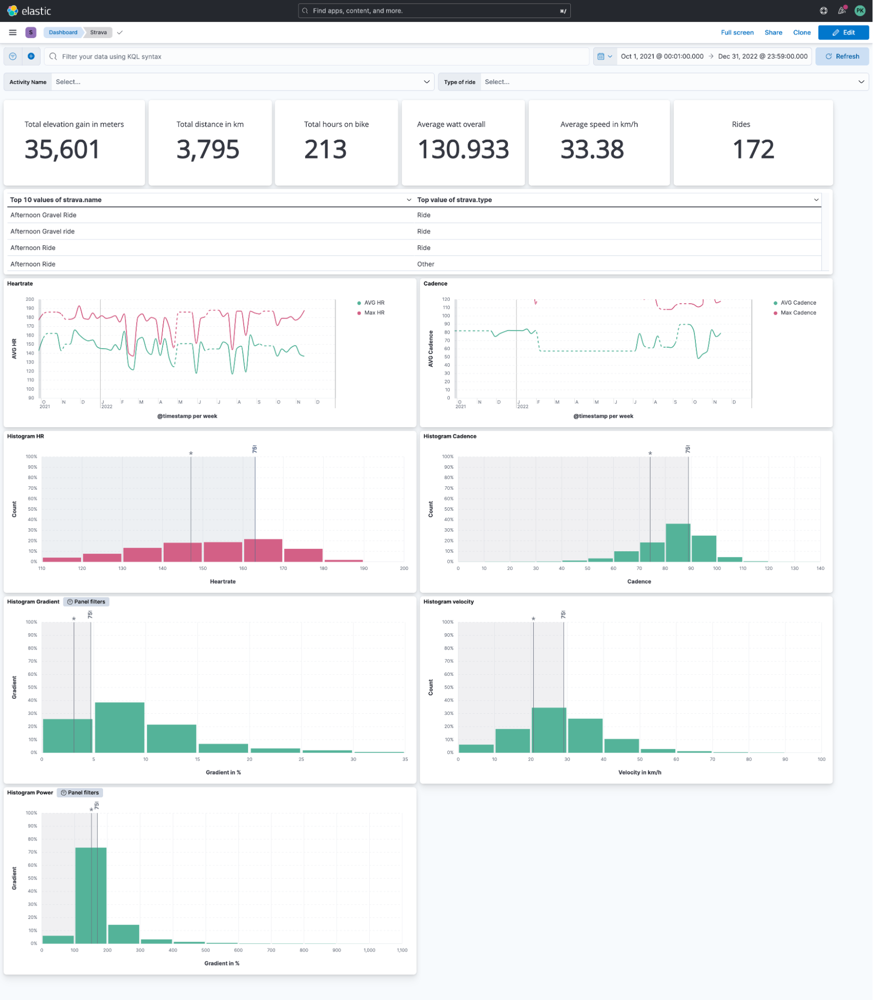
Strava does not provide the ability to view all activities in a single view. Do you want to know your average heart rate overall rides in the last month? You can swap heart rate with any available stream, like cadence!
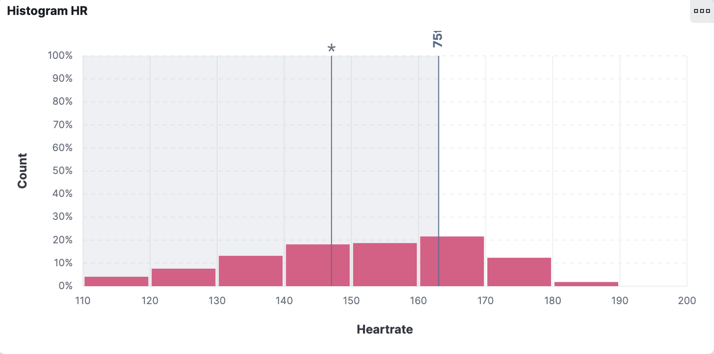
I like to view my data in a histogram view because it gives me a good overview of the distribution. This histogram shows me the heart rate distribution. Our visualization tool allows us to add reference lines, which can be a static value, based on aggregation, or anything else as a formula. The first line with the asterisk (*) symbol tells me my average heart rate overall rides combined. The second line shows me the 75% percentile, meaning I was below 75% of all my time on a bike.
This is interesting as it translates to how you should train, whether you are doing enough base workouts or you tend to ride hard all the time and shift the histogram towards higher numbers.
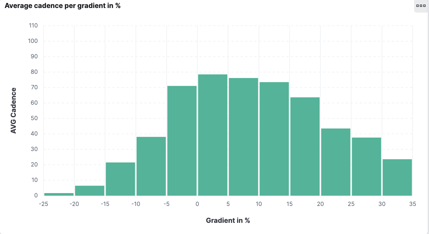
Another fascinating thing that Elasticsearch allows us to do is a more explorative view. Cadence is described as the revolution per minute — that is, how many full turns of your crank are you performing? In layman's terms, how often does your foot do a full rotation?
Is there a relationship between cadence and gradient? Indeed the steeper it gets, the lower the cadence must drop. I always wonder if the actual data support my perception. Using Lens, we can put the gradient as a % value on the horizontal axis and the cadence on the vertical axis. It immediately catches your eye that there is a sudden drop in the 20%+ range.
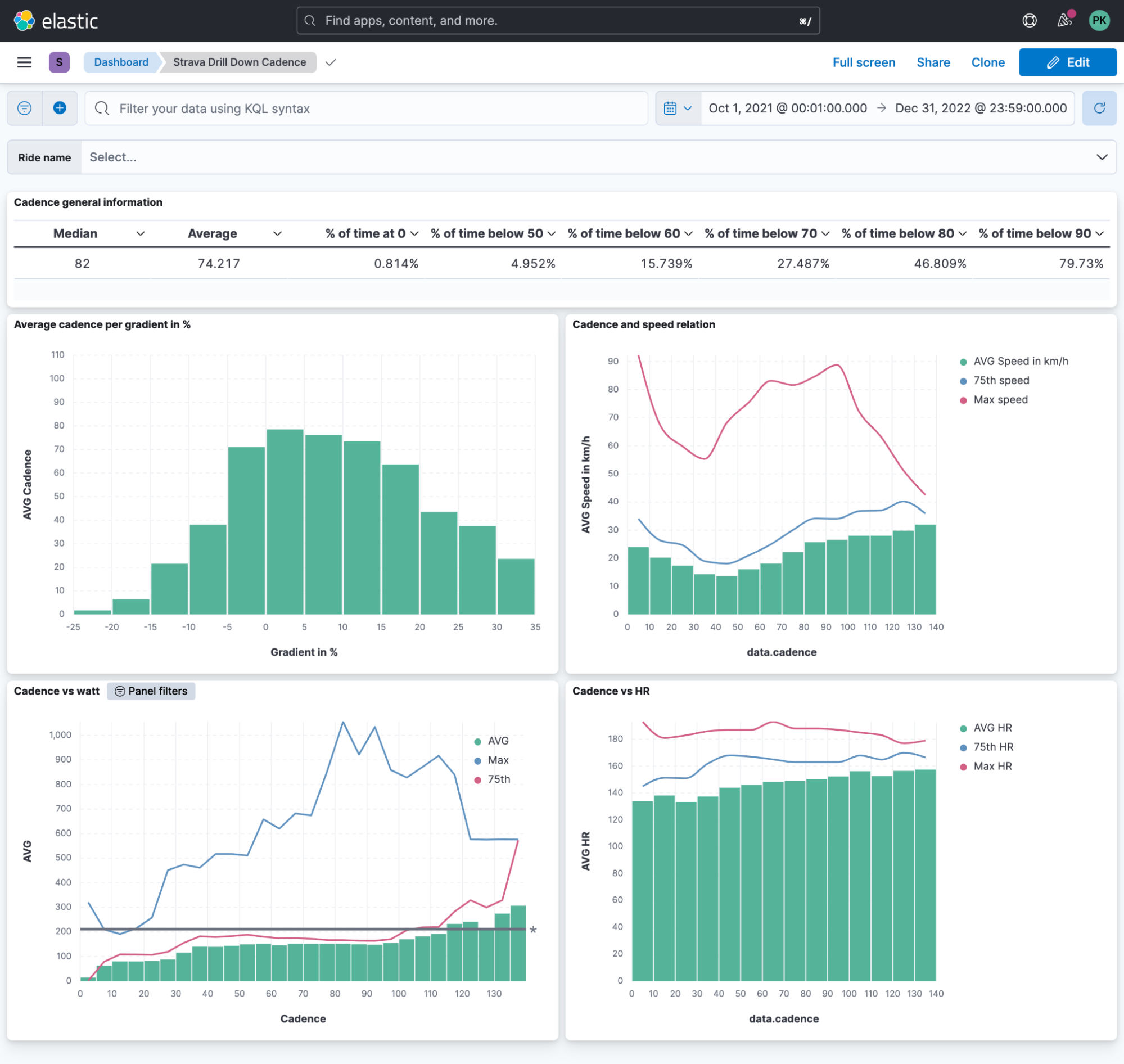
Summary
We achieved quite a bit in this blog post, and you can start exploring your data now! I’ll leave you with a dashboard I built featuring all possible information I can think of for cadence data.
Ready to get started? Begin a free 14-day trial of Elastic Cloud. Or download the self-managed version of the Elastic Stack for free.
Check out the other posts in this Strava series:
- Part 1: How to import Strava data into the Elastic Stack
- Part 3: Get more out of Strava activity fields with runtime fields and transforms
- Part 4: Optimizing Strava data collection with Elastic APM and a custom script solution
- Part 5: How tough was your workout? Take a closer look at Strava data through Kibana Lens
- Part 6: Unlocking insights: How to analyze Strava data with Elastic AIOps
- Part 7: From data to insights: Predicting workout types in Strava with Elasticsearch and data frame analytics
Share
- Share on Twitter
Share on Twitter
- Share on LinkedIn
Share on LinkedIn
- Share on Facebook
Share on Facebook
- Share by Email
Share by Email
- Print this page
Print