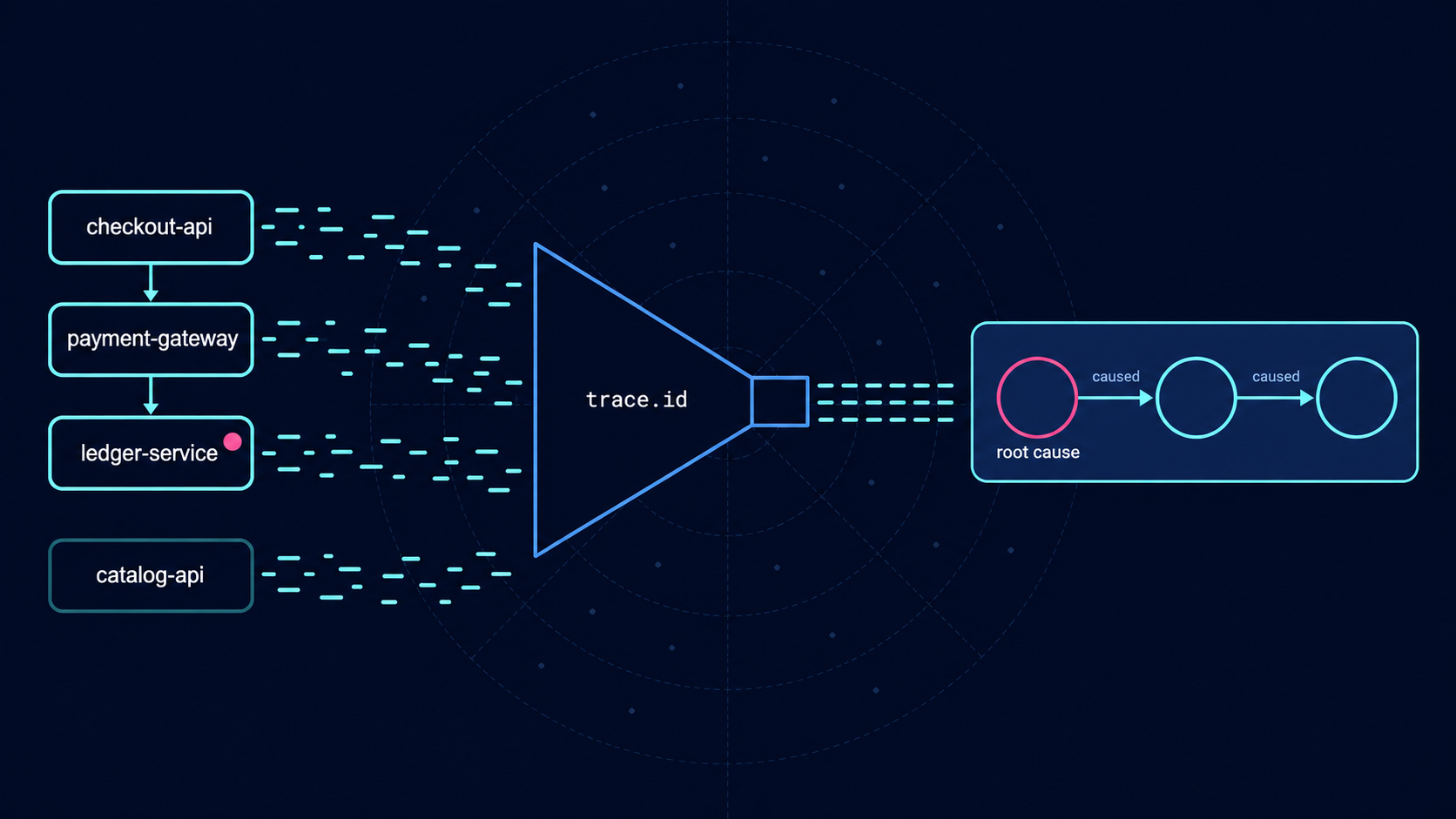
Your trace stops at the span; continuous profiling with OpenTelemetry doesn’t

Elastic speaks OpenTelemetry natively. Send traces, logs, and metrics over OTLP straight into Elasticsearch, no proprietary agents required. See how it fits together, try it for free in the cloud, or run it locally.

Continuous profiling is now an OpenTelemetry (OTel) signal, and Elastic can collect it from an application that you never touch. The OpenTelemetry Profiling integration uses eBPF to sample every process on a Linux host, so CPU profiling runs without any code changes or restarts. In our lab, an unmodified Spring PetClinic served 30,150 requests in four minutes on a little over half a CPU core. The flamegraph resolved those samples into Spring Data repository calls and Hibernate queries, as well as H2 result processing. The integration is a technical preview. We install it through Fleet and read the flamegraph in Kibana. Then we query the stored samples with Elasticsearch Query Language (ES|QL).

Prerequisites: kernel, Elastic Agent version, and permissions

• Kibana and Elastic Agent 9.4 or later. This is a Fleet-managed OpenTelemetry input package: Elastic Agent runs in its default mode and manages the OTel Collector's profiling receiver and Elasticsearch output for you.

• A Linux host running kernel 5.10 or newer on amd64 or arm64. The profiler uses eBPF, a Linux mechanism for running verified programs in the kernel, and needs the corresponding host permissions. It samples processes across the host without application code changes or restarts.

• A superuser account the first time, to initialize Universal Profiling storage.

You can find the companion notebook here. It reproduces the whole example from this article, including creating the policy and querying the samples, along with the steps in between, and cleaning up.

What continuous profiling shows that a trace doesn’t

A trace follows a request through instrumented operations, while a CPU profile samples the active stack: the chain of function calls executing at that moment. Because collection is continuous, it also includes background threads and code that never got a span:

Note that this preview collects CPU profiles only; it doesn’t provide a heap or allocation profile.

Profiles entered OpenTelemetry Alpha in March 2026 and remain Alpha as of September 15, 2026, so Elastic's integration 0.0.1 is a technical preview. Our Profiles Alpha article covers the work behind that milestone.

How to set up continuous profiling with OTel

The whole setup is a Fleet policy and an enrolled agent.

Step 1: Initialize Universal Profiling storage

The integration writes into the same profiling-* indices that Universal Profiling reads, so those indices have to exist first. If your deployment has never used Universal Profiling, open Infrastructure > Universal Profiling and select Set up Universal Profiling. This needs a superuser and is a one-time step per deployment.

Step 2: Create a profiling policy in Fleet

In Integrations, search for OpenTelemetry Profiling and select Add OpenTelemetry Profiling.

Note: If the integration doesn’t show up, switch your space's solution view to Observability and then search again. In the classic view, Kibana hides technical preview integrations from the catalog.

Give the integration a name, and keep its receiver enabled. Expand Change defaults and then Advanced options to set samples_per_second; we'll use 20. Choose a new agent policy, and leave Collect system logs and metrics unchecked so the flamegraph only contains the profiler's data. Then select Save and continue.

Step 3: Enroll your Linux agent

Select Add Elastic Agent to your hosts, and follow the enrollment instructions for your platform. For Docker, use the official Elastic Agent container procedure with Linux host process visibility and the profiler's required eBPF permissions. The screenshots use Elastic Agent 9.5.3 in a Linux ARM64 virtual machine (VM) running kernel 6.10.14, profiling an unmodified Java demo.

Step 4: Confirm that the agent is healthy and sending samples

In Fleet > Agents, open the new agent and confirm that it’s Healthy and lists the profiling integration:

Generate some traffic against PetClinic (the notebook runs a four-minute loop of owner searches, owner pages, and the vets list), and then check the flamegraph for that time window. Agent health alone doesn’t confirm that samples arrived. 

Step 5: How to read a flamegraph and find CPU work

Open Infrastructure > Universal Profiling > Flamegraphs, and select the traffic window. Then filter to the application:

process.executable.name : "java"

The samples resolve into Java functions, including Spring Data repository calls and Hibernate queries, as well as H2 result processing.

Note: The profiler resolves Java frames by reading the HotSpot Java Virtual Machine’s (JVM's) internal structures, so the application has to run on a regular JVM. A GraalVM native image, such as the published spring-petclinic container image, still gets its CPU samples counted, but each stack stops at a single native frame.

How to read a flamegraph:

• Width is the signal. Wider frames account for more of the samples in the window that you selected.

• Vertical stacking is the call chain. Callers sit below, and callees are above.

• Horizontal position means nothing. This isn’t a timeline; a frame on the left isn’t earlier than the one on the right.

• Start wide, and then narrow. Follow the widest branch down or search for one of your own functions, and zoom in.

This capture is a four-minute synthetic burst, so compare a steady traffic window before deciding what to optimize. Also keep in mind what a sample means: a sampled database call shows CPU executing in that stack. It doesn’t measure the time spent waiting on the database.

Step 6: Query CPU profiling samples with ES|QL

The profiles are regular documents, so we can query them. In Discover, select the same time window and then run:

FROM profiling-events-all
| WHERE process.executable.name == "java"
| STATS samples = SUM(Stacktrace.count)
  BY minute = BUCKET(@timestamp, 1 minute)
| SORT minute

Stacktrace.count is the number of CPU samples stored in each event, so the query returns a sample count per minute. In this run, it returns 691, 644, 715, 664, and 131 samples across five buckets; the traffic ran for four minutes, so the first and last buckets are partial. The notebook gets the same numbers from the ES|QL API.

The profiler samples each CPU core 20 times per second, so one fully busy core adds up to 1,200 samples per minute. On our six-vCPU host, PetClinic kept a little over half of one core busy while serving 30,150 requests in four minutes. Note that these counts aren’t milliseconds or CPU percentages: 

Connect profiles to traces and CPU metrics

The OpenTelemetry Profiles data model supports associations with trace_id and span_id. With compatible instrumentation and correlation configured, a slow span can lead you to its sampled CPU stacks. The profiling package alone doesn’t instrument requests or complete that setup. Our trace-to-profile correlation walk-through shows how it works with the Elastic Distribution of OpenTelemetry (EDOT) Java on Stack 8.13; correlation with this preview package needs separate validation.

For CPU trends by runtime or kernel category, the profilingmetricsconnector turns stacks into OTel time-series counters, such as hotspot.count and kernel.count. The connector runs in your own OTel Collector pipeline; it isn’t part of this package's generated configuration, and its dashboards ship as a separate Kibana integration. Once you have a baseline, those counters can feed ES|QL, dashboards, and machine learning (ML) anomaly detection. You can learn more about this connector in this article from Observability Labs.

Where to start with continuous profiling

With the OpenTelemetry Profiling integration, adding the fourth signal is a Fleet policy and a container with the right permissions. It requires no code changes or restarts, and the profiles land in the same Universal Profiling views and ES|QL that you currently use. Start with a service that you already investigate through logs and metrics, as well as application performance monitoring (APM), and add its CPU profile. Find the recurring work, and compare the same workload after a change.

The integration is a technical preview on top of an Alpha signal, so expect the package and the data model to change. The companion notebook creates the policy and runs the lab, as well as cleans it up, so you can repeat the whole exercise on a newer version in a few minutes.