Elasticsearch has native integrations with the industry-leading Gen AI tools and providers. Check out our webinars on going Beyond RAG Basics, or building prod-ready apps with the Elastic vector database.
To build the best search solutions for your use case, start a free cloud trial or try Elastic on your local machine now.
Machine learning pipelines have evolved tremendously in the past several years. With a wide variety of tools and frameworks out there to simplify building, training, and deployment, the turnaround time on machine learning model development has improved drastically. However, even with all these simplifications, there is still a steep learning curve associated with a lot of these tools. But not with Elastic.
In order to use machine learning in the Elastic Stack, all you really need is for your data to be stored in Elasticsearch. Once there, extracting valuable insights from your data is as simple as clicking a few buttons in Kibana. Machine learning is baked into the Elastic Stack, allowing you to easily and intuitively build a fully operational end-to-end machine learning pipeline. And in this blog, we’ll do just that.
Why Elastic?
Being a search company means that Elastic is built to efficiently handle large amounts of data. Searching and aggregating data for analysis is made simple and intuitive using Elasticsearch Query DSL. Large data sets can be visualized in a variety of ways in Kibana. The Elastic machine learning interface allows for easy feature and model selection, model training, and hyperparameter tuning. And after you’ve trained and tuned your model, Kibana can also be used to evaluate and visually monitor models. This makes the Elastic Stack the perfect one-stop shop for production-level machine learning.
Example data set: EMBER 2018
We’re going to demonstrate end-to-end machine learning in the Elastic Stack using the EMBER data set, released by Endgame to enable malware detection using static features derived from portable executable (PE) files. For the purpose of this demonstration, we will use the EMBER (Endgame Malware BEnchmark for Research) 2018 data set, which is an open source collection of 1 million samples. Each sample includes the sha256 hash of the sample file, the month the file was first seen, a label, and the features derived from the file.
For this experiment, we will select 300K samples (150K malicious and 150K benign) from the EMBER 2018 data set. In order to perform supervised learning on the samples, we must first select some features. The features in the data set are static features derived from the content of binary files. We decided to experiment with the general, file header and section information, strings, and byte histograms in order to study model performance on using different subsets of features of the EMBER data set.
End-to-end machine learning in the Elastic Stack: A walkthrough
For the purposes of this demo, we will use the Python Elasticsearch Client to insert data into Elasticsearch, Elastic machine learning’s data frame analytics feature to create training jobs, and Kibana to visually monitor models after training.
We will create two supervised jobs, one using general, file header and section information, and strings, and another using just byte histograms as features. This is to demonstrate simultaneous multiple model training in the Stack and visualization of multiple candidate models later.
Elasticsearch setup
In order to use machine learning in the Elastic Stack, we first need to spin up Elasticsearch with a machine learning node. For this, we can start a 14-day free trial of Elastic Cloud that is available for anyone to try. Our example deployment has the following settings:
- Cloud Platform: Amazon Web Services
- Region: US West (N. California)
- Optimization: I/O Optimized
- Customize Deployment: Enable Machine Learning
We also need to create API keys and assign them appropriate privileges to interact with Elasticsearch using the Python Elasticsearch Client. For our walkthrough, we will be inserting data into the ember_ml index, so we’ll create a key as follows:
Data ingest
Once we have our Elasticsearch instance set up, we’ll begin by ingesting data into an Elasticsearch index. First, we will create an index called ember_ml and then we will ingest the documents that make up our data set into it using the Python Elasticsearch Client. We will ingest all the features required for both models into a single index, using the Streaming Bulk Helper in order to bulk ingest documents into Elasticsearch. The Python code to create the ember_ml index and bulk ingest documents into it is as follows:
Note that the feature vectors need to be flattened, i.e., each feature needs to be a separate field of a supported data type (numeric, boolean, text, keyword, or IP) in each document, since data frame analytics does not support arrays with more than one element. Also notice that the “appeared” (first seen) field in the EMBER data set has been altered to match an Elasticsearch-compatible date format for the purpose of making time series visualizations later.
To make sure that all our data is ingested in the right format into Elasticsearch, we run the following queries in the Dev Tools Console (Management -> Dev Tools):
To get count of the number of documents:
To search for documents in the index and make sure they’re in the right format:
Once we have verified that the data in Elasticsearch looks as expected, we are now ready to create our analytics jobs. However, before creating the jobs, we need to define an index pattern for the job. Index patterns tell Kibana (and consequently the job) which Elasticsearch indices contain the data that you want to work with. We create the index pattern ember_* to match our index ember_ml.
Model training
Once the index pattern is created, we’ll create two analytics jobs with the two subsets of features, as mentioned above. This can be done via the Machine Learning app in Kibana. We will configure our job as follows:
- Job type: We select “classification” to predict whether a given binary is malicious or benign. The underlying classification model in Elastic machine learning is a type of boosting called boosted tree regression, which combines multiple weak models into a composite model. It uses decision trees to learn to predict the probability that a data point belongs to a certain class.
- Dependent variable: “label” in our case, 1 for malicious and 0 for benign.
- Fields to include: We select the fields we would like to include in the training.
- Training percentage: It is recommended that you use an iterative approach to training, especially if you’re working with a large data set (i.e., start by creating a training job with a smaller training percentage, evaluate the performance, and decide if it is necessary to increase the training percentage). We’ll start with a training percentage of 10% since we are working with a sizable data set (300K documents).
- Additional information options: We’ll leave the defaults as they are, but you can choose to set hyperparameters for the training job at this stage.
- Job details: We’ll assign an appropriate job ID and destination index for the job.
- Create index pattern: We’ll disable this, since we will be creating a single index pattern to match the destination indices for both our training jobs in order to visualize the results together.
We’ll create two analytics jobs following the process described above, one with only the bytes histogram as features (destination index: bytes_preds) and one with everything but byte histogram as features (destination index: main_preds). The analytics job determines the best encodings for each feature, best performing features, and optimal hyperparameters for the model. The job progress can also be tracked in the Machine Learning app:

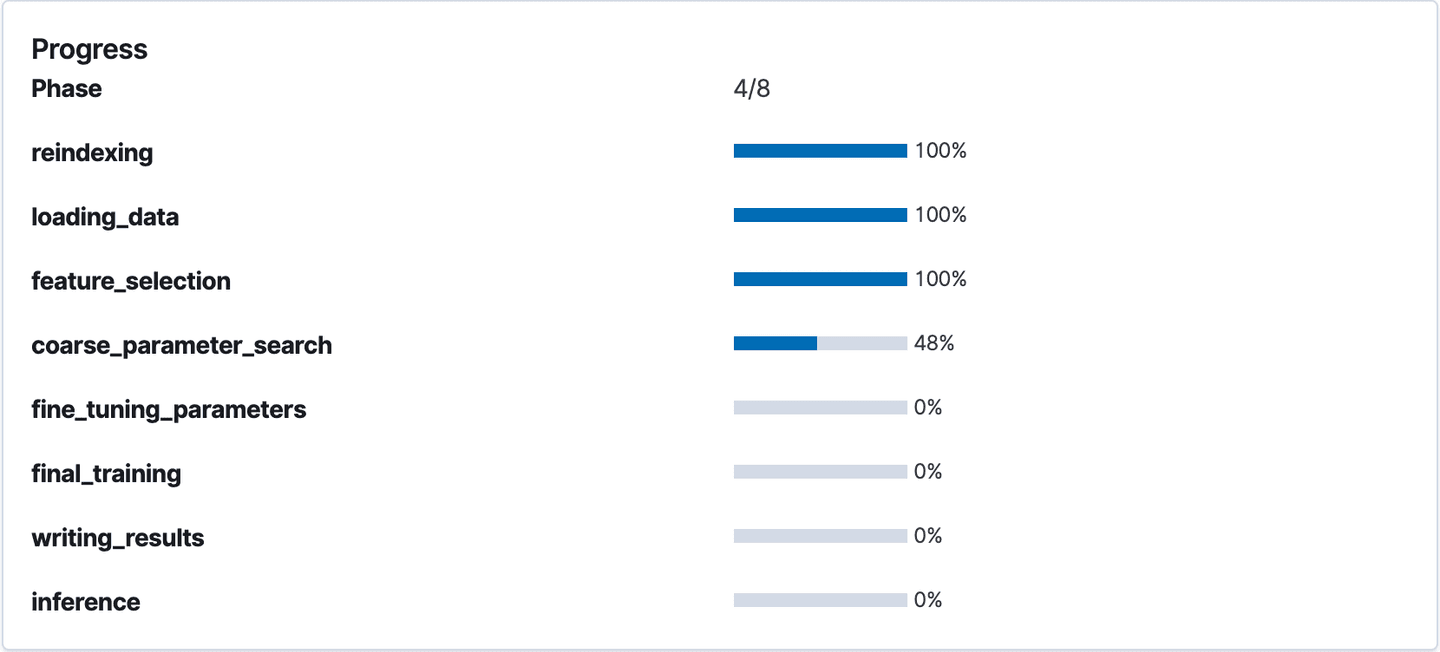
Tracking job progress in the Machine Learning app
Model evaluation
Once the jobs have completed, we can view the prediction results by clicking the View button next to each of the completed jobs. On clicking View, we see a dataframe-style view of the contents of the destination index and the confusion matrix for the model. Each row in the dataframe (shown below) indicates whether a sample has been used in training, the model prediction, label, and class probability and score:

Dataframe view of the main_preds destination index
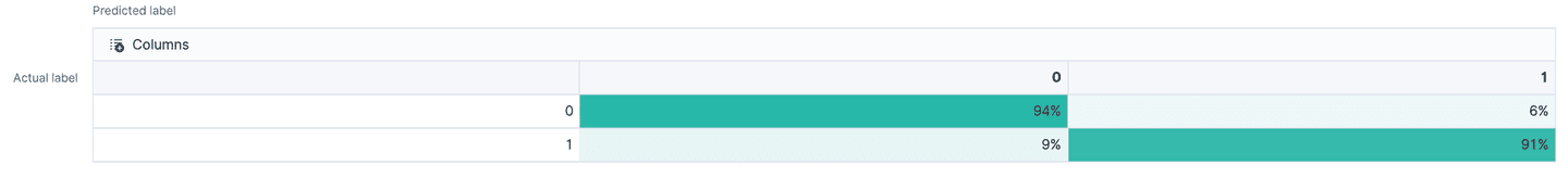
We use the confusion matrices to evaluate and compare the performance of both the models. Each row in the confusion matrix here represents instances in the actual class and each column represents instances in the predicted class, thus giving a measure of true positives, false positives (top row), false negatives, and true negatives (bottom row).

Confusion matrix for model with general, file header and section information, and strings as features
Confusion matrix for model with byte histogram as features
We see that both models have pretty good accuracy (at least for the purposes of a demo!) so we decide against another round of training or hyperparameter tuning. In the next section, we will see how to visually compare the two models in Kibana and decide which model to deploy.
Model monitoring
Once we have the predictions for both the models in their respective destination indices, we will create an index pattern (*_preds, in this case) to match the two in order to create model monitoring dashboards in Kibana. For this example, the monitoring dashboard serves two purposes:
- Compare the performance of the byte histogram-only model with the other model; we use TSVB visualizations for this.
- Track different metrics for the better performing model; we use vertical bar visualizations to visualize prediction probabilities and benign vs malicious sample counts as well as TSVB to track false positive rate and false negative rate.
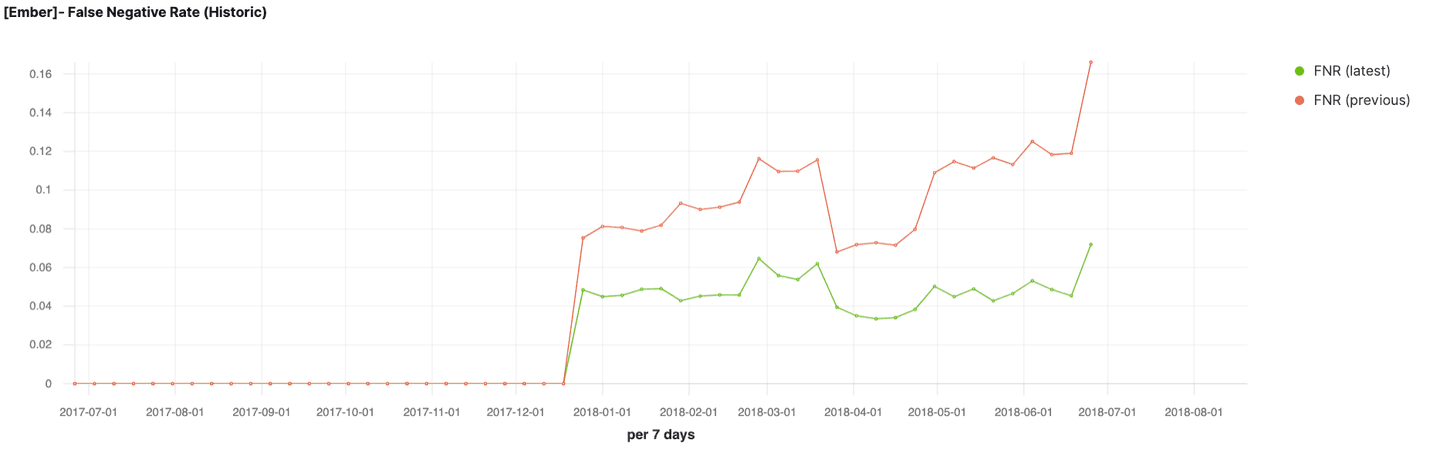

False negative rate and false positive rate of the two trained models over time
By observing the false negative rate and false positive rate of the two models across a significant time range, and looking at the confusion matrices shown in the previous section, we conclude that the model trained on general, file header and section information, and strings is the better performing model. We then plot various metrics that we would like to track for this model, assuming this is the one we want to deploy and monitor post-deployment.
Dashboard of various model performance metrics created in Kibana
In real-world use cases, such monitoring dashboards can be used to compare candidate models for production and once a model has been deployed, identify indicators of model decay (e.g., false positive bursts) in production environments and trigger relevant responses (e.g., new model training). In the next section, we’ll see how to deploy our chosen model for use in a machine learning production pipeline.
Deploying our supervised model to enrich data at ingest time
In addition to model training and evaluation, the Elastic Stack also provides a way for a user to use trained models in ingest pipelines. This in turn opens up an avenue to use machine learning models to enrich your data at ingest time. In this section, we will take a look at how you can do exactly this with the malware classification model we trained above!
Suppose that in this case we have an incoming stream of data extracted from binaries that we wish to classify as either malicious or benign. We will ingest this data into Elasticsearch through an ingest pipeline and reference our trained malware classification model in an inference processor.
First, let’s create our inference processor and ingest pipeline. The most important part of the inference processor is the trained model and its model_id, which we can look up with the following REST API call in the Kibana console:
This will return a list of trained models in our cluster and for each model, display characteristics such as the model_id (which we should make a note of for inference), the fields used for training the model, when the model was trained, and so forth.

Sample output from a call to retrieve information about trained models shows the model_id, which is required for configuring inference processors
If you have a large number of trained models in your cluster, it might be helpful to run the API call above with a wildcard query based on the name of the data frame analytics job that was used to train the model. In this case, the models we care about were trained with jobs called ember_*, so we can run
to quickly narrow down our models to the desired ones.
Once we have made note of the model_id, we can create our ingest pipeline configuration. The full configuration is shown below. Make a note of the configuration block titled inference. It references the model we wish to use to enrich our documents. It also specifies a target_field (which in this case we’ve set to is_malware, but can of course be set according to preference), which will be used to prefix the ML fields that will be added when the document is processed by the inference processor.
Now suppose we are ingesting documents with features of binaries and we wish to enrich this data with predictions of the maliciousness of each binary. An abridged sample document is shown below:
We can ingest this document by using one of the Index APIs and pipe through the malware-classification pipeline we created above. An example API call that ingests this document into a destination index called main_preds is shown below. To save space, the document has been abridged.
As a result, in our destination index main_preds, we now have a new document that has been enriched with the predictions from our trained machine learning model. If we view the document (for example, using the Discover tab), we will see that per our configuration, the inference processor has added the predictions of the trained machine learning model to the document. In this case, our document (which represents an unknown binary we want to classify as malicious or benign) has been assigned class 1, which indicates that our model predicts this binary to be malicious.

A snippet from the ingested document shows enrichment from our trained machine learning model
As new documents with predictions are added to the destination index, these will automatically be picked up by the Kibana dashboards, thus providing insight into how the trained model is performing on new samples over time.
Conclusion
In production environments, the buck does not (or should not!) stop with model deployment. The pipeline needs to have a way to effectively evaluate models before they reach the customer environment and monitor them closely once they are deployed. This helps data science teams foresee issues in the wild and take necessary action when there are indicators of model decay.
In this blog post, we explored why the Elastic Stack is a great platform for managing such an end-to-end machine learning pipeline, given that it has great storage capabilities, model training, built-in tuning, and an exhaustive suite of visualization tools in Kibana.
Related Content
July 7, 2026
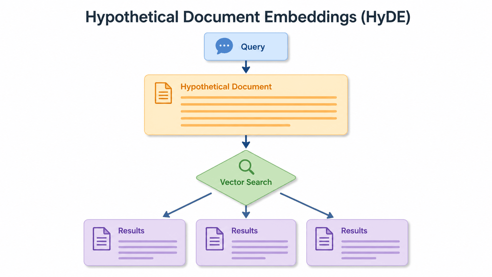
Short queries, formal documents: how HyDE improved semantic search precision by 50% in Elasticsearch
HyDE boosts semantic search precision and recall by 50% on short queries. Here's how to implement it in Elasticsearch with the Inference API and semantic_text.
June 24, 2026
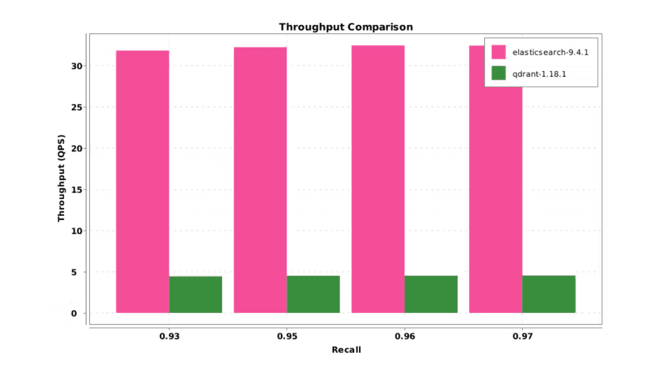
Elasticsearch DiskBBQ delivers 7x faster vector search than Qdrant on network-attached storage
Elasticsearch DiskBBQ achieves up to 7x higher vector search throughput than Qdrant at comparable recall on network-attached storage. Explore the benchmark methodology and full results.
July 6, 2026
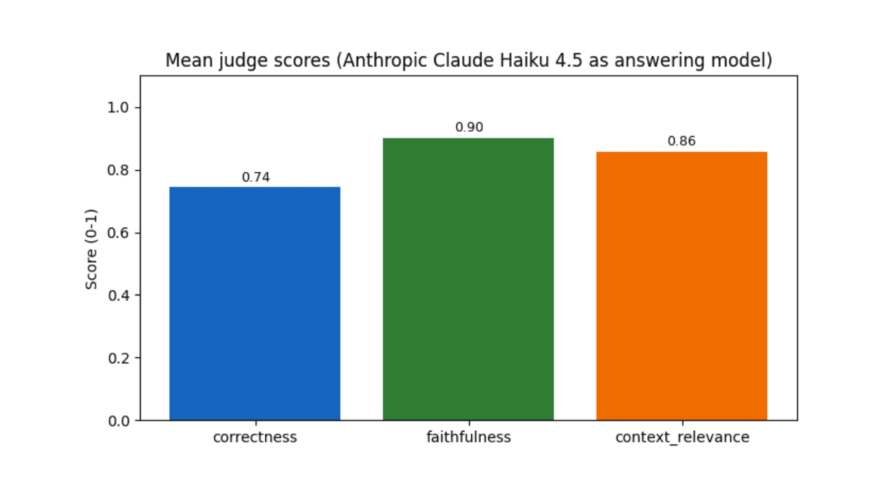
Who grades the grader? LLM-as-a-Judge inside Elasticsearch Workflows
Find out if your RAG agent is ready to ship. Score it on correctness, faithfulness and retrieval quality using only Elasticsearch Workflows and two Claude models.

June 15, 2026
Your search index is already an agent memory system: Persistent agent memory for Claude Code with Elasticsearch
Give your AI agent persistent cross-session memory using Elasticsearch: Hybrid recall, a knowledge graph, and cross-device handoffs. Three commands to install.

June 15, 2026
Your FAQ bot doesn't need a PhD: LLM query routing with Elastic Workflows
Route LLM queries by complexity using Elasticsearch search metadata: Mistral Small for FAQ questions, Claude Sonnet for multi-source synthesis.