Cooking up machine learning models: A deep dive into the supervised learning pipeline


 Share on Twitter
Share on Twitter

 Share on LinkedIn
Share on LinkedIn

 Share on Facebook
Share on Facebook

 Share by Email
Share by Email

 Print this page
Print
Have you ever heard the saying "cooking is like science"? Well, the same could be said for machine learning. Just like cooking, building a machine learning (ML) pipeline requires a series of precise steps, a dash of creativity, and a good understanding of the ingredients you're working with.
Don't have the time, skills, or knowledge? Or are you tired of spending hours in the kitchen chopping, mixing, and blending ingredients by hand? Imagine being able to automate the entire cooking process with the push of a button. That's what you can do with an Elastic ML supervised learning job!
Just like a cooking food processor, the machine learning pipeline in Elasticsearch streamlines the process of making accurate predictions and automating decision-making. This blog post will take a closer look at the different stages of a data frame analytics supervised learning job in Elastic Stack. It also describes the secret sauce that allows users with no machine learning expertise to train accurate models. The curious reader will find specifics and implementation details of the advanced machine learning techniques we use. So grab your apron, and let's get started!
The supervised learning pipeline
Let's first look at what happens when you create a supervised learning job. Once you have started a classification or regression job and look at the job details tab in the Data Frame Analytics Jobs view, you can see the following training phases.
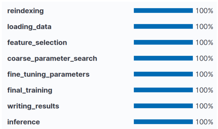
This visualization allows the user to see the progress of the job, even if a job takes a significant amount of time.
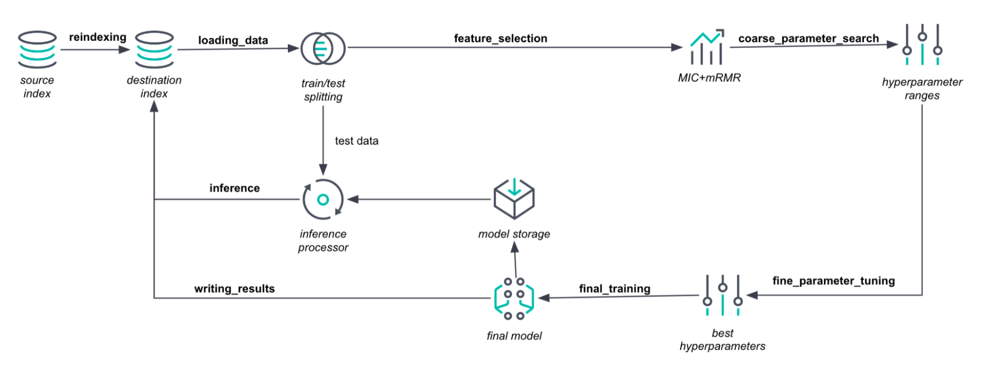
Data preprocessing
We start with reindexing , copying the selected data into the destination index. Then in the loading_data phase, the data is passed to the Java process. It is divided into training and test data sets. To keep the datasets representative, we use problem-dependent sampling methods like stratification. The training dataset is then passed to feature selection.
In the feature_selection phase, we compute a variant of the maximum information coefficient (MIC) with minimum redundancy maximum relevancy (mRMR). Thus, we estimate the dependencies between the features and the target values. We look at three types of encodings for categorical fields: one-hot encoding, target mean encoding, and frequency encoding. We then rank the features and encodings that are more and less important for predicting the target.
As a result, we get the (encoded) features together with their sampling probabilities. The higher the sampling probability for a feature, the more often it will be selected into the feature bag when we generate a new tree. Simply put, if MIC tells us that one feature is twice as important as another, we will use it twice as often when creating a data subset to generate a new tree.
Hyperparameter optimization
If hyperparameters are not set in the job configuration, we search for the best values. By definition, many hyperparameters can be set to any positive number. This leads to infinite search intervals, which are impossible to search.
Hence, in the coarse_parameter_searchphase, we limit the search intervals for the unspecified hyperparameters. We sample several values for a selected hyperparameter. Then solve a quadratic optimization problem to find the most promising search interval. We fix the hyperparameter value at best seen one and move on to the next hyperparameter.To evaluate hyperparameters, we use the cross-validation error and choose the number of folds based on the amount of data available. To speed up this process for large datasets, we use a single split into training and validation sets. Here we would use less than 50% of the data for training.
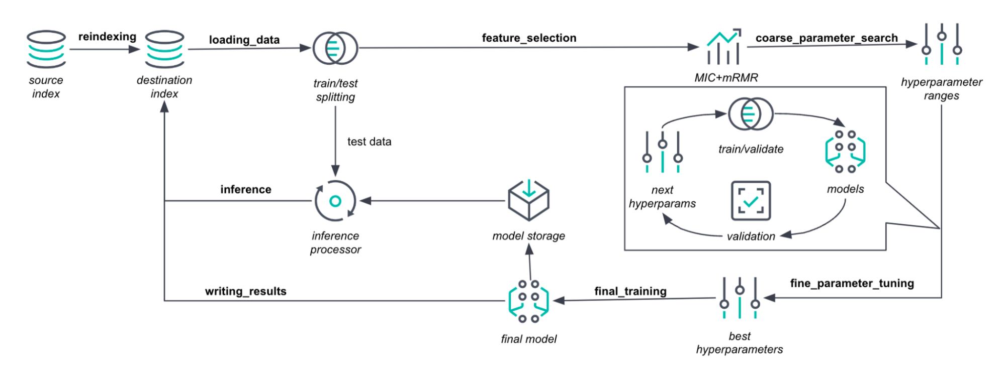
With the finite intervals determined, we proceed to the fine_tuning_parameters phase. Here, we run a Bayesian optimization procedure guided by Expected Improvement. Inside Bayesian optimization, we create a Gaussian process that describes the relationship between the model hyperparameters and the model accuracy. This is the most time-consuming phase of a job. If the early_stopping job parameter is enabled (as it is by default), we can reduce the tuning time. To this end, we use ANOVA decomposition of the Gaussian process. It tells us when the gain from an optimization step is indistinguishable from the noise.
Final training and evaluation
In the final_training phase, the optimal hyperparameters and all training data are used to train the final model. This leads to more efficient and accurate models, especially for small- and medium-sized datasets. The final model then computes predictions and feature importance values.
In the writing_results phase, the model and predictions are stored in Elasticsearch indices. The model is stored as a compressed JSON document in the model definitions index. The predictions and feature importances are stored in the destination index.
Finally, in the inference phase, the inference processor evaluates the test set. The results are also stored in the destination index.
Conclusion
The future of machine learning for search is just a whisker away with Elastic ML! So grab your mixing spoon, preheat your data, and start building your own machine learning masterpieces. Start your free Elastic Cloud trial today to access the platform. Happy cooking!
Share
- Share on Twitter
Share on Twitter
- Share on LinkedIn
Share on LinkedIn
- Share on Facebook
Share on Facebook
- Share by Email
Share by Email
- Print this page
Print