Get hands-on with Elasticsearch: Dive into our sample notebooks in the Elasticsearch Labs repo, start a free cloud trial, or try Elastic on your local machine now.
Welcome to the future of music information retrieval, where machine learning, vector databases, and audio data analysis converge to deliver exciting new possibilities! If you're interested in the world of music data analytics or merely passionate about how technology is revolutionizing the music industry, this guide is for you.
Here, we will take you on a journey of searching music data using an approach known as vector search. Since more than 80% of our world data is unstructured, it is good to know how to treat different kinds of data other than text.
If you want to follow and execute the code while reading, access the file on GitHub listed at the end of this article.
The architecture
Imagine if you could hum the tune of a song you're trying to recall, and suddenly the song you hummed appears on the screen? Of course, given the necessary effort and data model tuning, that's what we're going to do today.
To achieve our result, we will create an architecture as shown below:

The main actor here is the embeddings. We will use the audio embedding generated by a model to use as a search key in our vector search.
How to generate an audio embedding
At the core of generating embeddings are models that are trained on millions of examples to deliver more relevant and accurate results. For audio, these models can be trained on a vast amount of audio data. The output of these models is a dense numeric representation of the audio (i.e., the audio embedding). This high-dimensional vector captures key characteristics of the audio clip, allowing for similarity computations and efficient searches in the embedded space.
For that job, we will use librosa (open source python package) to generate audio embeddings. This typically involves extracting meaningful features from audio files, such as Mel-frequency cepstral coefficients (MFCCs), chroma, and mel-scaled spectrogram features. So, how can we implement audio search with Elasticsearch®?
Step 1: Creating an index to store audio data
First things first, we need to create an index in Elasticsearch before populating our vector database with our music data.
- Begin by deploying Elasticsearch (we have a 14-day free trial for you).
- During the process, remember to store the credentials (username, password) to be used in our Python code.
- For simplicity, we will use Python code running on a Jupyter Notebook (Google Collab).
1.1 Create our audio data set index
Now that we have a connection, let's create an index that will store audio information.
The provided Python code uses the Elasticsearch Python client to create an index with specific configurations. The aim of the index is to provide a structure that allows for search operations on dense vector fields, which are typically used to store vector representations or embeddings of some entity (such as audio files in this case).
The index_config object defines the mapping properties of this index, including fields for "audio-embedding", "path", "timestamp", and "title". The "audio-embedding" field is specified as a "dense_vector" type, accommodating for a dimensionality of 2048, and is indexed with "cosine" similarities, which dictate the method used to calculate the distance between vectors during search operations. The "path" field will store the path to play the audio. Note that to accommodate an embedding dimensionality of 2048, you'll need to use Elasticsearch version 8.8.0 or later.
The script then checks whether an index exists in the Elasticsearch instance. If the index does not exist, it creates a new index with the specified configuration. This type of index configuration can be used in scenarios such as audio search, where audio files are transformed into vector representations for indexing and subsequent similarity-based retrieval.
Step 2: Populating Elasticsearch with audio data
At the end of this step, you will have an index read to be filled with audio data to create our datastore. So that we can proceed with audio search, we first need to populate our database.
2.1 Selecting audio data to ingest
Numerous audio data sets have specific objectives. For our example, I will utilize files generated on the Google Music LM page, specifically from the Text and Melody Conditioning section. Put your audio files *.wav in a specific directory — in this case, I choose my GoogleDrive "/content/drive/MyDrive/audios".
The code defines a function named list_audio_files that takes a directory as an argument. This function aims to traverse through a provided directory and its subdirectories, looking for audio files with the extension “.wav”. The function would need to be modified if support for .mp3 files is desired.
2.2 The power of embeddings for vector search
This step is where the magic happens. Vector similarity search is a mechanism to store, retrieve, and search for vectors based on their similarity given a query, commonly used in applications such as image retrieval, natural language processing, recommendation systems, and more. This concept is widely used due to the rise of deep learning and the representation of data using embeddings. Essentially, embeddings are vector representations of high-dimensional data.
The fundamental idea is to represent data items (e.g., images, documents, user profiles) as vectors in a high-dimensional space. Then, the similarity between vectors is measured using a distance metric, such as cosine similarity or Euclidean distance, and the most similar vectors are returned as the search results. While text embeddings are extracted using linguistic features, audio embeddings are often generated using spectrograms or other audio signal features.

The process of creating embeddings for both text and audio data involves transforming the data into vectors using a feature extraction or embedding technique and then indexing these vectors in the vector search database.
2.2.3 Extracting the audio features
The next step involves analyzing our audio files and extracting meaningful features. This step is critical as it helps the machine learning model to understand and learn from our audio data.
In the context of audio signal processing for machine learning, the process of feature extraction from spectrograms is a crucial step. Spectrograms are visual representations of the frequency content of audio signals over time. The identified features in this context encompass three specific types:
- Mel-frequency cepstral coefficients (MFCCs): MFCCs are coefficients that capture the spectral characteristics of audio signals in a manner more closely related to human auditory perception.
- Chroma features: Chroma features represent the 12 distinct pitch classes of the musical octave and are particularly useful in music-related tasks.
- Spectral contrast: Spectral contrast focuses on the perceptual brightness of different frequency bands within an audio signal.
By analyzing and comparing the effectiveness of these feature sets in real-world text files, researchers and practitioners can gain valuable insights into their suitability for various audio-based machine learning applications, such as audio classification and analysis.
- First, we will need to convert our audio files into a suitable format for analysis. Libraries like
librosain Python can help with this conversion, turning the audio files into spectrograms. - Next, we will extract features from these spectrograms.
- Then, we will save these features and send them as inputs for our machine learning model.
We are using panns_inference, which is a Python library designed for audio tagging and sound event detection tasks. The models used in this library are trained from PANNs, which stands for Large-Scale Pretrained Audio Neural Networks, a method for audio pattern recognition.
Note: It may take a few minutes to download the PANNS inference model.
2.3 Insert audio data into Elasticsearch
Now we have everything we need to insert our audio data into the Elasticsearch index.
2.4 Visualizing the results in Kibana
At this point, we can check our index with audio data embedded in an audio-embedding dense-vector field. Kibana® Dev Tools, particularly the Console feature, is a powerful interface for interacting with your Elasticsearch cluster. It provides a way to directly send RESTful commands to Elasticsearch and view the results in a user-friendly format.

Step 3: Searching by music
Now, you can perform vector similarity search using the generated embeddings. When you provide an input song to the system, it will transform the song into an embedding, search the database for similar embeddings, and return songs with similar features.
Let's start with the fun part!
3.1 Selecting music to search
In the code below, we select music directly from GitHub audios directory and use the Audio music to play the result inside Google Colab.
You can play the music by clicking Play.

3.2 Searching the music
Now, let's run a code to search for that music "my_audio " inside Elasticsearch. We will use only the audio file for search.
And Elasticsearch will return you all the music similar to your key song:
A little code to help play the results:
Now, you can check the result by clicking Play.
3.3 Analyzing the results
So, can I deploy this code in a production environment and sell my app? No, as a probabilistic model, the Probabilistic Auditory Neural Network (PANN), and any other machine learning models, require an increased volume of data and additional fine-tuning to be effectively applied in real-world scenarios.
This is made evident by the graph visualizing the embeddings associated with our sample of 18 songs, which can cause false positives for a kNN approach. However, a notable challenge persists for future data engineers: the task of identifying the optimal model for query by humming. This represents a fascinating intersection of machine learning and auditory cognition, which calls for rigorous research and innovative problem-solving.

3.4 Improving the POC with a UI (optional)
With a little modification, I copied and pasted this entire code to Streamlit. Streamlit is a Python library that simplifies creating interactive web applications for data science and machine learning projects. It allows newcomers to easily turn data scripts into shareable web apps without extensive web development knowledge.
The result is this app:
A window to the future of audio search
We have successfully implemented a music search system using Elasticsearch vectors in Python. This serves as an initial point in the field of audio search and could potentially inspire more innovative concepts by utilizing this architectural approach. By altering the models, it is possible to develop diverse applications. Additionally, porting the inference to Elasticsearch could potentially enhance the performance. Visit Elastic’s machine learning page to learn more about it.
This indicates the considerable potential and adaptability of this technology for a variety of search applications beyond text.
All the code is available in a single Google Colab file, elastic-music_search.ipynb, on GitHub.
References
- What is unstructured data?
- Music Classification: Beyond Supervised Learning, Towards Real-world Applications
- Deploy Elasticsearch in 3 minutes or less
- How vector similarity search works
- Getting Started With Embeddings
- PANNs inference
- A faster way to build and share data apps
- Musicinformationretrieval.com
- PANNs: Large-Scale Pretrained Audio Neural Networks for Audio Pattern Recognition
Related Content

June 18, 2026
Jingra: A Reproducible Framework for Vector Search Benchmarking
Jingra is an open source benchmarking framework that runs the same vector search workload across Elasticsearch, OpenSearch and Qdrant so you can compare engines under identical, reproducible conditions.
June 16, 2026
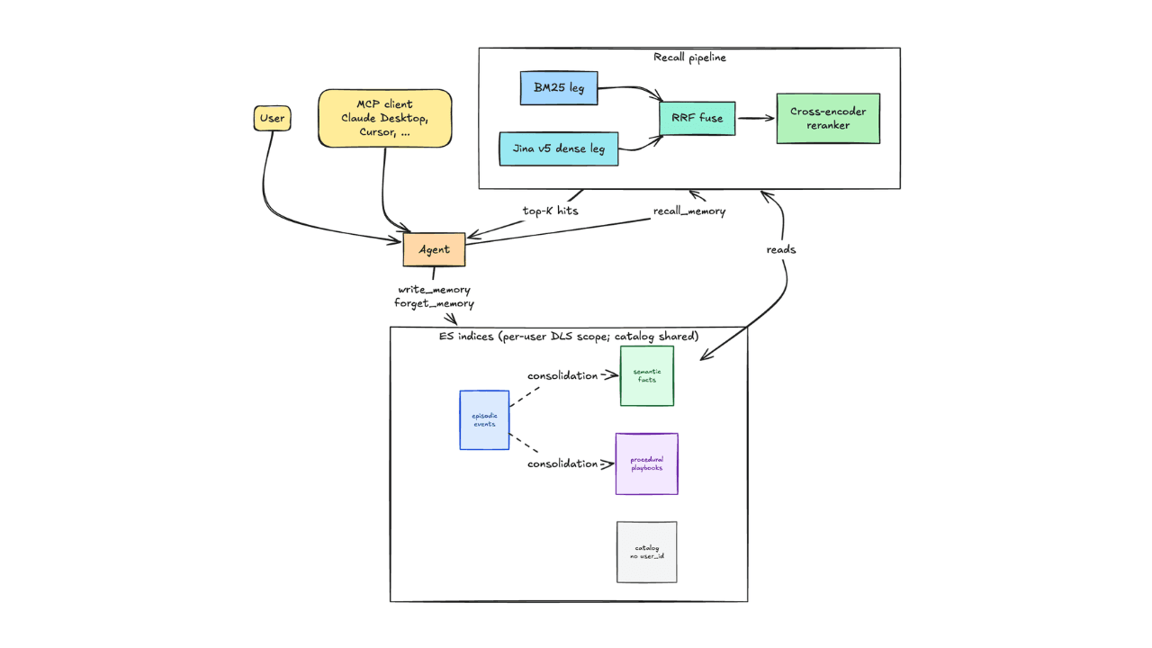
How we built a persistent agent memory layer on Elasticsearch with 0.89 recall and zero tenant leaks
Discover the architecture behind a persistent, multi-tenant agent memory layer on Elasticsearch: three indices, hybrid retrieval with RRF and a reranker, supersession, decay, and per-user DLS isolation. R@10 0.89 across 168 questions. Full open-source implementation included.
June 10, 2026
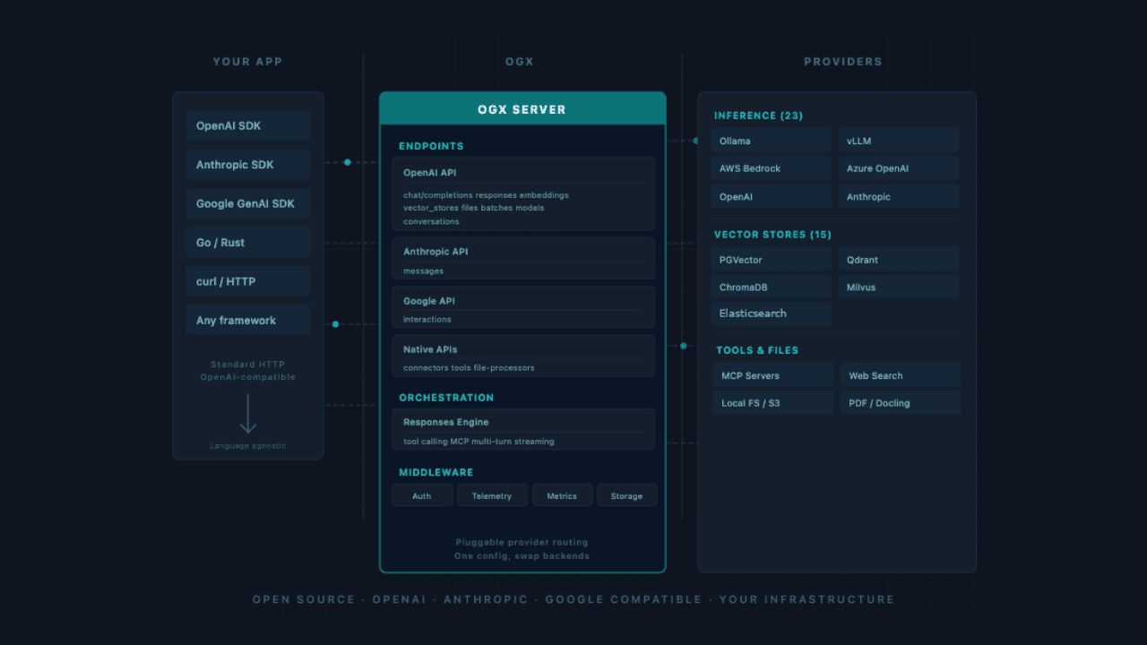
Your AI agent reads the fine print: building a RAG pipeline over EU regulations with Elasticsearch and OGX
Learn how to configure Elasticsearch as an OGX vector store, ingest EU regulation PDFs and build a Python RAG agent that runs hybrid BM25 and vector search with source-level citations.

June 9, 2026
Best practices for building a modern app with vector search
Exploring six vector search tips for building modern AI search applications entirely on Elasticsearch, with an opinionated rationale at each architectural decision.
June 8, 2026
Elasticsearch simdvec deep-dive: Walking the memory tightrope to 2x better vector throughput
A deep dive into four optimizations (cascade unrolling, batch prefetching, dim-axis unrolling, a structural refactor) that pushed Elasticsearch simdvec to 2x vector throughput by working with the CPU, not against it.