Parsing and enriching log data for troubleshooting in Elastic Observability

In an earlier blog post, Log monitoring and unstructured log data, moving beyond tail -f, we talked about collecting and working with unstructured log data. We learned that it’s very easy to add data to the Elastic Stack. So far the only parsing we did was to extract the timestamp from this data, so older data gets backfilled correctly. 

We also talked about searching this unstructured data toward the end of the blog. While unstructured data can be incredibly useful when combined with full text search functionality, there are cases where we need a little more structure to use the data to answer our questions.

Schema on write or schema on read — why not both?

Schema on write remains the default option that Elasticsearch uses to handle incoming data. All fields in a document are indexed as it’s ingested, otherwise known as schema on write. This is what makes running searches in Elastic so fast, regardless of the volume of data returned or the number of queries executed. It’s also a big part of what our users love about Elastic.

Schema on write works really well if you know your data and how it’s structured before ingest. That way, the schema (logical view of data structure) can be fully defined in the index mapping. It also requires sticking to that defined schema when queries are run against the index. In the real world, however, monitoring and telemetry data can often change. New data sources may appear in your environment, for example. An added layer of flexibility to dynamically extract or query new fields after the data has been indexed adds tremendous value, even if it comes at a slight cost to performance. 

That’s where schema on read comes in. Data can be quickly ingested in raw form without any indexing, except for certain necessary fields such as timestamp or response codes. Other fields can be created on the fly when queries are run against the data. You don’t need to have intimate knowledge of your data ahead of time, nor do you have to predict all the possible ways that the data may eventually be queried. You can change the data structure at any time, even after the documents have been indexed — a huge benefit of schema on read.

Here’s what’s unique about how Elastic has implemented schema on read. We’ve built runtime fields on the same Elastic platform — the same architecture, the same tools, and the same interfaces you’re already using. There are no new datastores, languages, or components, and there’s no additional procedural overhead. Schema on read and schema on write work well together and seamlessly complement each other, so that you can decide which fields to calculate when a query requires them and which fields to index when your data is ingested into Elasticsearch. 

By offering you the best of both worlds on a single stack, we make it easy for you to decide which combination of schema on write and schema on read works best for your specific use cases.

Using runtime fields on the Elastic Stack

Let us start with a quick example.

Using unstructured data we can easily answer questions like “How many errors did we have in the last 15 minutes?” or “When did we last have error X?” But if we want to ask questions like “What’s the sum of number X that appears in our logs?” or “What are our top 5 errors?”, then we need to extract the relevant information first in order to aggregate. 

If you’ve followed along with our last blog, our data in the cluster now looks like this:

If we’d like to sum up how many ads our service served up, we need to extract the numeric value of these log messages first.

The easiest way to do this is to use runtime fields. This functionality allows you to define additional fields in your documents even if they did not exist in the original value that you sent to Elasticsearch. 

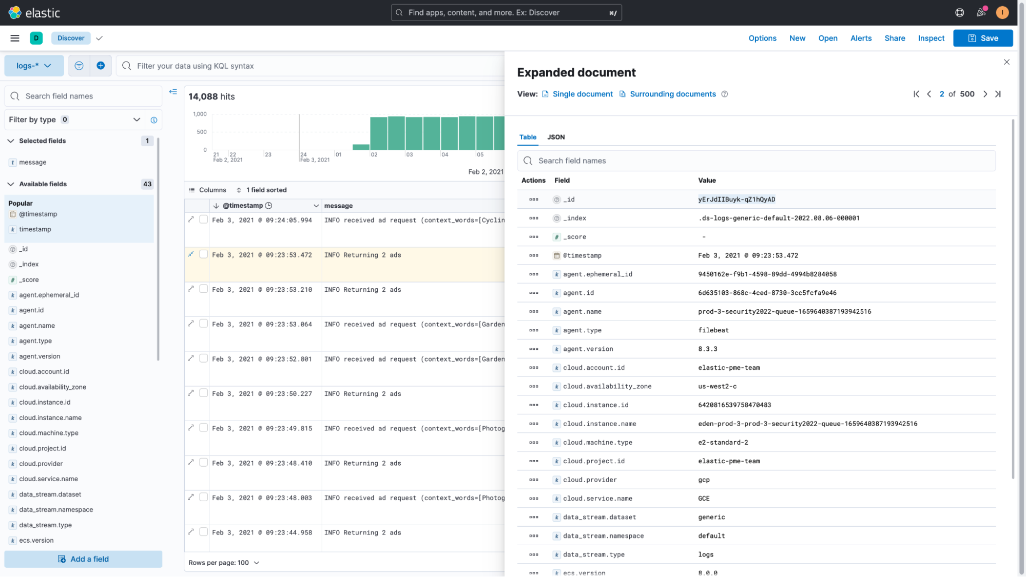
To do this query, let’s start out in the Discover UI where we will select one of our documents that has the log message that we’d like to parse. After opening the document details, we will copy the document “_id.” This is an important step to make script writing a little bit easier.

[Related article: Runtime fields: Schema on read for Elastic]

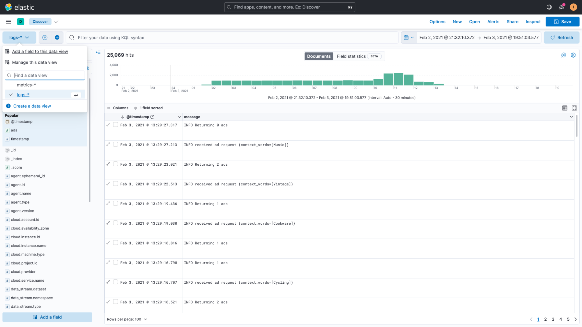
Next, we’ll click on the name of the index pattern or dataview (logs-* in our case) and then click on “Add a field to this data view.”

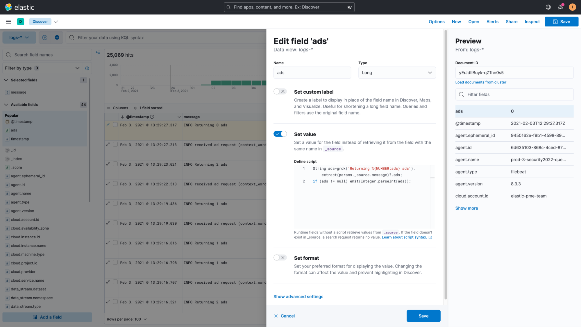
This will open a flyout that lets us create our runtime field. On the top right, we will paste the document ID that we copied earlier. This document is then loaded and the script will run against this document and provide instant results, so we can see if our attempt worked or not. 

Next we’ll give the new field a name. Then we will select “Set value” from the available options. Instead of just setting a static value, this option will allow us to write a script. 

The script required to parse the message field is:

It’s a relatively simple painless script. The most important components are “grok,” which allow us to run any GROK expression against our data, similar to how we handle the timestamp extraction in the earlier blog.

Since this is a grok expression, we temporarily save the extracted data in a field that we call “ads.” 

grok('Returning %{NUMBER:ads}

The expression is being run on the field “message.”

.extract(params._source.message)

And once executed we access the temporary “ads” field like this:

?.ads;

Toward the end of the script, we then check if we were able to successfully extract the value. If yes, we emit it.

if (ads != null) emit(Integer.parseInt(ads));

The most important thing to remember is that you have to use .extract(params._source.message) when using runtime fields against “text” fields, and .extract(doc[“message”]).

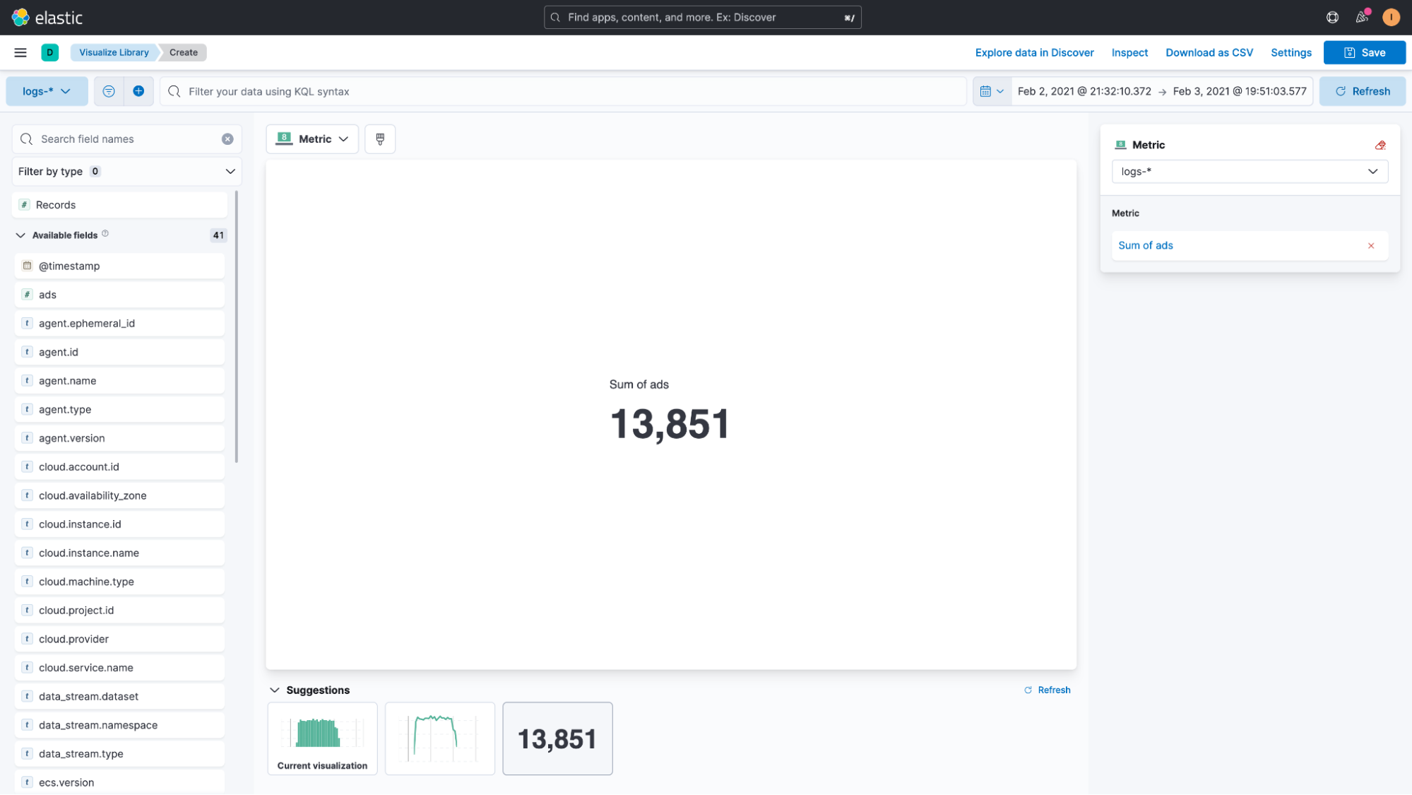
With the field added to Kibana, we can now start looking at our data in Discover again. If everything worked correctly, we can then use this field as we would any other field — using it in a Lens visualization is just one example of that.

These runtime fields can also be used for filtering, so we can search for “ads:1” in our example to limit the documents to only those where a single ad was returned. The fields really do behave as if they exist in our documents as part of an existing schema.

The benefits of runtime fields

Because runtime fields aren’t indexed, adding a runtime field doesn’t increase the index size. You define runtime fields directly in the index mapping, saving storage costs and increasing ingestion speed. When you define a runtime field, you can immediately use it in search requests, aggregations, filtering, and sorting, without the additional need to re-index your data.

The downside of runtime fields

Every time you run a search against your runtime fields, Elasticsearch has to evaluate the field’s value again since it’s not a real field in your documents that gets indexed. If this field is one that you intend to query frequently in the future, then you should consider extracting it as part of your ingest pipeline. 

If the data you extracted from your documents is only being used once in a while, then you can safely continue to use the runtime field functionality. However, if you plan on using the field often or if you notice performance issues, then it’s probably a good idea to just add it to the ingest pipeline that we’ve defined in the earlier blog, Log monitoring and unstructured log data, moving beyond tail -f.

Runtime fields for non-Kibana users

If you’re not using Kibana to explore your data or want to use this same functionality in your custom applications, then you can also map these runtime fields in the mapping of your indices.

The way they will be computed will stay the same. That means that even if you define them in the mapping, the potentially heavy work of extracting them will have to be done at search time. However, since they are defined in your index mapping, you can use them with custom queries and aggregations by directly accessing Elasticsearch. 

An example of this would look as follows:

And you can find more information about this approach in our documentation: Map a runtime field.

In this blog, we’ve learned how easy it is to use runtime fields on already indexed data. We did not have to re-index a single document but were still able to query and analyze our data as if we’ve had the field all along. This feature in Elastic Stack saves time and allows for more powerful ad hoc analyses and data exploration.

Stay tuned as we next tackle data visualizations and dashboards to take advantage of your rich logging data! In the meantime, check out our Logging Quick Start training resources to learn more.