Search relevance from click streams: Using Learn To Rank and behavioral signals with OpenTelemetry

Every click on a search result is an implicit relevance judgment, and conversions are a stronger signal. The search analytics you've been capturing through OpenTelemetry contain the behavioral data to improve search relevance. Techniques start simple, with fixes you can ship this week and build toward Learn To Rank (LTR) models trained on real click data. The instrumentation that surfaces problems also generates the training data to fix them.

What you'll discover

In this post, you'll learn how to:

• Build judgment lists from click data to evaluate and improve relevance.

• Apply basic search tuning (field weights, boosts, query rules) informed by analytics.

• Create rank features from behavioral signals, like popularity and conversion rate.

• Understand LTR and how click data becomes training data.

• Close the feedback loop between analytics and relevance improvement.

What you'll need

• Search analytics data from the previous blogs in this series (search, click, and conversion spans in Elastic).

• An Elasticsearch index with product data (the reference project includes sample data with rank features).

• Familiarity with Elasticsearch queries (BM25 [Elasticsearch's default text scoring algorithm], rank_feature, function scores).

Search relevance techniques at a glance

From search analytics to search relevance improvements

Over the past three posts, you built a full instrumentation pipeline, including search spans with search.* attributes and click tracking with position data and click-through rate (CTR) / Mean Reciprocal Rank (MRR) metrics. This pipeline also includes conversion spans tying searches to revenue. And it all sits in traces-generic.otel-default, queryable with Elasticsearch Query Language (ES|QL).

Now you have dashboards, and you know that your CTR is 28%. You also know which queries generate revenue and which ones users abandon. Plus, you can tell your product manager exactly where the funnel leaks.

Now what?

The real value of search analytics is using behavioral data to improve relevance and close feedback loops. It’s also important to make search learn from its users. Your experience tells you that measurement is necessary but not sufficient, and a dashboard that shows poor ranking doesn't improve that ranking. 

This post covers four practical areas:

1. Judgment lists: The foundation for evaluating and improving relevance.

2. Basic search tuning: Field weights, boosts, and query rules informed by analytics.

3. Rank features for personalization: Feeding behavioral signals back into ranking.

4. LTR: Training machine learning (ML) models on click data to optimize ranking automatically.

Each one draws directly from the search.* attributes you're already collecting, and they don’t require any new instrumentation.

What are judgment lists?

Before diving into specific techniques, it's worth understanding the concept that ties them all together: judgment lists.

A judgment list is a set of query-document pairs with relevance grades: For a given query, how relevant is each document? They look like this:

Judgment lists serve three purposes:

• Evaluating current relevance. Given a set of queries and known-good results, how well does your search rank them? Metrics like Normalized Discounted Cumulative Gain (NDCG) and the Rank Eval API use judgment lists to score your ranking quality. This gives you a baseline before making changes.

• Measuring the impact of changes. When you adjust field weights or add synonyms, judgment lists tell you whether the change helped or hurt. The same is true when you change boosting rules. Run the same evaluation before and after: If NDCG went up, the change improved relevance for those queries.

• Training LTR models. LTR algorithms need labeled training data, such as, For this query, these documents are relevant and those aren't. Judgment lists are that training data.

Manual vs. automated judgment lists

Traditionally, judgment lists are created by human assessors who manually rate documents for a set of test queries. This works well for a small number of high-value queries (your top 50 searches, for example), but it doesn't scale. A large catalog with thousands of distinct queries and frequent inventory changes makes manual assessment impractical.

This is where your click data becomes valuable. Every click is an implicit relevance judgment; that is, a signal that for a given query, a given document was relevant enough to engage with. Conversions are even stronger signals. By aggregating this data, you can build judgment lists automatically from real user behavior, at a scale that manual assessment can't match.

The trade-off is noise. Clicks are influenced by position bias (users click higher-ranked results more often regardless of relevance) and presentation effects. They’re also influenced by accidental clicks. We'll cover techniques to handle this noise later in this post. But the key insight is that approaches like personalization and LTR lean toward automated judgment lists because it's not scalable to manually create lists for every query or user segment, nor for every inventory change.

The judgment lists guide on Search Labs covers the concept in depth, including how to structure lists for evaluation with the Rank Eval API.

How search analytics identify search relevance problems

The most immediate use of your analytics data is to identify and fix specific relevance problems. This only requires using data to direct manual improvements, no personalization or ML.

Finding problem queries with search analytics

The ES|QL queries from the click in your application give you per-query CTR and MRR. Sort by search volume descending and CTR ascending to find your highest-impact relevance failures:

FROM traces-generic.otel-default
| WHERE ((name == "search" AND attributes.search.query IS NOT NULL)
    OR attributes.search.first_click == true)
  AND attributes.search.query IS NOT NULL
| STATS
    searches = COUNT(CASE(name == "search" AND attributes.search.query IS NOT NULL, 1)),
    clicked = COUNT(CASE(attributes.search.first_click == true, 1))
  BY attributes.search.query
| EVAL ctr_pct = ROUND(100.0 * clicked / searches, 1)
| WHERE searches > 5
| SORT ctr_pct ASC, searches DESC
| LIMIT 20

This is the CTR-by-query query re-sorted to surface problems first. The WHERE searches > 5 filter removes one-off queries that would dominate the low-CTR list with small sample noise.

• Zero-CTR queries with results.  Your ranking is returning content, but none of it’s compelling. These queries often benefit from synonym expansion. You can also improve them with boosting rules or pinned results.

• Low-CTR, high-volume queries. These are the biggest relevance investment opportunities, and they affect the most users.

• Low-MRR, high-CTR queries. Users find what they need but have to scroll for it. In these instances, the relevant documents exist, but they're ranked wrong.

Try it: Close the loop in the reference project

If you have click data in the reference project(python generate_traffic.py --blog 3 --sessions 100), you can run the problem-query query above against traces-generic.otel-default and observe your lowest-CTR queries.

The reference project's app.py already uses rank_feature boosting: rank_features.popularity, rank_features.conversion_rate, rank_features.margin_score, and rank_features.freshness are indexed on every product and blended into the BM25 score at query time. To see the effect of adjusting a boost:

1. Open reference/app.py, and find the "should" clause in _build_search_query().

2. Change the "boost" value on rank_features.popularity from 2 to 5.

3. Restart the server (python app.py) and rerun generate_traffic.py --blog 3 --sessions 50.

4. Compare the top-queries and click position distribution in ES|QL before and after.

This is informed manual tuning using the behavioral data you collected, not ML. That's the pattern for the rest of this post: First, ES|QL tells you what's wrong. Then, configuration changes and, eventually, LTR models fix it.

Field weights, boosts, and scoring for search relevance

The simplest tuning lever in Elasticsearch is adjusting how different fields contribute to the relevance score. A multi_match query across title, description, and brand fields can weight the title higher because a match there is usually more relevant. Your analytics data tells you where these weights are wrong: If users consistently click products with titles that don't match the query but with descriptions that do, your title boost may be too aggressive.

Beyond field weights, you can incorporate business metrics directly into scoring. A common example is boosting by profit margin; that is, products with higher margins rank slightly higher when relevance scores are similar. The rank_feature field type is designed for exactly this: Index a numeric signal (margin, popularity, recency) alongside each document, and the rank_feature query blends it with text relevance at query time. For more complex scoring combinations, like decay functions, weighted field values, and scripts, the function_score query gives you full control. The boosting by profit and popularity guide on Search Labs walks through this in detail, including the trade-offs between additive and multiplicative boosting approaches.

Query rules for targeted search relevance fixes

For targeted interventions, query rules let you pin, boost, or exclude specific results for specific queries, and no model training is required. They're the search equivalent of a manual override.

Your analytics data tells you exactly where to apply them. When you see a zero-CTR query, like "returns policy", that consistently returns product results instead of the returns page, you can pin the returns page at position 1 for that query. If you notice a high-revenue query where the best-selling product appears at position 4, you can boost it.

Query rules are valuable precisely because they're simple. They solve known problems immediately while you build toward more sophisticated approaches. The query rules tutorial on Search Labs walks through the setup.

Building judgment lists from click data

The basic tuning above handles individual problems. To improve relevance systematically, you need judgment lists, and your click data can build them automatically.

Converting click data into relevance grades

The simplest approach is to count clicks per query-document pair and assign graded relevance:

FROM traces-generic.otel-default
| WHERE attributes.search.action == "click"
  AND attributes.search.query IS NOT NULL
| STATS
    click_count = COUNT(*),
    avg_position = AVG(attributes.search.result_click_position)
  BY attributes.search.query, attributes.search.result_click_id
| SORT attributes.search.query, click_count DESC

This gives you a table of (query, document, click_count, avg_position) tuples. The grading step maps click counts to relevance levels:

The thresholds depend on your traffic volume. For a high-traffic site, you might need 10+ clicks before calling something "highly relevant." For lower traffic, even two or three clicks is a meaningful signal. The point is that click frequency across users is a stronger signal than any single click.

You can strengthen judgments further by incorporating conversion data, a document that gets clicked and added to cart is a stronger relevance signal than one that gets clicked and abandoned:

FROM traces-generic.otel-default
| WHERE attributes.search.action IN ("click", "add_to_cart")
  AND attributes.search.query IS NOT NULL
| STATS
    clicks = COUNT(CASE(attributes.search.action == "click", 1)),
    carts = COUNT(CASE(attributes.search.action == "add_to_cart", 1))
  BY attributes.search.query, attributes.search.result_click_id
| SORT attributes.search.query, clicks DESC

A document with five clicks and three cart additions is a stronger candidate for grade 3 than one with five clicks and zero cart additions.

Handling position bias in click data

There's a problem with raw click counts: position bias. Users click position 1 more often because they see it first, not necessarily because it's the most relevant result. Blog 3 introduced this concept when we discussed click position distribution and referenced the foundational work by Joachims et al. (2005).

Position bias matters for judgment lists because it means raw click data over-weights whatever the current ranking happens to surface first. If you train an LTR model on biased judgments, it learns to replicate the existing ranking, which defeats the purpose.

Two practical approaches to handle this:

• Position-normalized click rates. Instead of raw click counts, calculate click-through rate per position. A document clicked 3 out of 10 times when shown at position 5 is arguably more relevant than one clicked 5 out of 10 times at position 1. Position 5 gets less visibility, so a higher click rate there is a stronger relevance signal.

• Skip-above heuristics. When a user clicks position 3 but skips positions 1 and 2, those skipped documents are implicitly judged "less relevant" for that query. This is the core insight from Joachims et al.: Skipped-above results provide negative training signals. You can extract these pairs from your click data:

FROM traces-generic.otel-default
| WHERE attributes.search.action == "click"
  AND attributes.search.query IS NOT NULL
| STATS
    min_click_position = MIN(attributes.search.result_click_position),
    max_click_position = MAX(attributes.search.result_click_position),
    click_count = COUNT(*)
  BY attributes.search.query_id, attributes.search.query
| WHERE min_click_position > 1
| SORT click_count DESC

Queries where the minimum click position is greater than 1 are sessions where the user skipped the top result(s). The documents at those skipped positions, for those queries, are candidates for grade 0 in your judgment list, because the user saw them and chose something lower.

For production judgment list generation, the LTR tutorial on Search Labs walks through the complete pipeline. The training LTR models with user behavior data guide covers the specific workflow of deriving training data from click-through behavior, including the Clicks Over Expected Clicks (COEC) algorithm for debiasing. And the LTR Jupyter notebooks provide working Python code for feature extraction and model training.

Rank features for search relevance personalization

Basic tuning applies the same ranking to every user. Personalization means adapting results based on who’s searching (their history, preferences, or segment). Rank features are the most accessible way to do this in Elasticsearch.

Building behavioral signals from click streams

You can aggregate your click and conversion data at the document level to produce signals that reflect overall or segment-specific popularity:

FROM traces-generic.otel-default
| WHERE attributes.search.action IN ("click", "add_to_cart")
| STATS
    clicks = COUNT(CASE(attributes.search.action == "click", 1)),
    carts = COUNT(CASE(attributes.search.action == "add_to_cart", 1))
  BY attributes.search.result_click_id
| EVAL cart_rate_pct = ROUND(100.0 * carts / clicks, 1)
| SORT clicks DESC
| LIMIT 20

These document-level signals (click popularity, cart rate, and conversion rate) are indexed as rank_feature fields on each product document. The workflow:

1. Run the ES|QL query above periodically (daily or weekly).

2. Write the results back to a click_popularity or conversion_rate rank_feature field on each product document.

3. Use a rank_feature query to blend text relevance with behavioral signals.

The rank_feature query applies a saturation function by default: Initial popularity gains matter most, diminishing as values get large. This prevents a single viral product from dominating all queries. You can tune the function's pivot point to control how much influence the feature has relative to text relevance.

Personalizing rank features by user segment

The query above produces global popularity; that is, it’s the same for every user. Personalization comes from segmenting these signals. If you're tracking enduser.pseudo.id or user.id, you can compute features per user cohort:

• Category affinity: How often does this user click products in "electronics" versus "clothing"?

• Price sensitivity: Does this user tend to click and convert on higher- or lower-priced items?

• Brand preference: Which brands does this user engage with most?

These become additional rank features, applied at query time based on who's searching. The personalized search with LTR guide on Search Labs walks through training per-user ranking models. For a lighter approach, the cohort-aware ranking guide shows how to use multiplicative boosting to personalize at the segment level without ML, just analytics-derived weights applied to rank features at query time.

Combining multiple signals with the linear retriever

When you're blending text relevance with semantic search and behavioral rank features, you need a way to combine them. Elasticsearch's linear retriever gives you precise control over how different query types contribute to the final ranking. It computes a weighted sum of normalized scores, so you can say text relevance matters 60%, semantic similarity 30%, popularity 10% and adjust those weights based on your analytics. This is unlike Reciprocal Rank Fusion (RRF), which only considers relative rank positions.

This is particularly useful for personalization because you can vary the weights per user segment. A returning customer might get more weight on purchase history, while a first-time visitor gets more weight on global popularity.

If you're also using semantic search with embedding models, the Elastic Inference Service (EIS) now offers GPU-accelerated embedding generation, including multilingual models, directly within Elastic Cloud, making it straightforward to add a semantic retriever alongside your text and behavioral signals.

How Learn To Rank uses click streams to optimize ranking

Rank features handle individual signals, but LTR handles all of them at once. It trains an ML model to combine features (like text relevance, popularity, CTR, recency, margin, or user affinity) into a single ranking function optimized for your users.

What you need for Learn To Rank in Elasticsearch

Elasticsearch has supported native Learning to Rank since version 8.12 as an Enterprise subscription feature. The pipeline:

1. Judgment list. Query-document pairs with relevance grades (built from click data, as above).

2. Feature extraction. Numeric signals for each query-document pair (BM25 score, popularity, CTR, recency, price, margin, user segment features).

3. Model training. Typically XGBoost or LambdaMART, trained on your judgment list with features.

4. Deployment. Upload the trained model to Elasticsearch via Eland, and use it as a rescorer.

The click and conversion data from this series feeds steps 1 and 2, and the judgment list is your training labels. The document-level features from the rank features section above (click popularity, conversion rate, margin) are additional features alongside text relevance scores.

Why automated judgment lists from click data scale better

This is where the scalability argument for automated judgment lists becomes concrete. A manually curated judgment list might cover your top 100 queries well, but personalized ranking needs judgment data across thousands of queries and multiple user segments. You can't hire assessors to rate results for "wireless headphones" separately for electronics enthusiasts, budget shoppers, and professional audio engineers.

Automated judgment lists from click data scale to every query your users actually run and update as inventory and user behavior change. They can also be segmented by cohort. The training LTR models with user behavior data guide demonstrates this end-to-end workflow, showing how to go from raw click events to trained ranking models.

For teams looking to close this loop even further, the agentic autotuning approach demonstrates using an AI agent to continuously monitor search quality and generate judgment lists from user interactions. It automatically retrains LTR models, turning the feedback loop into an autonomous system.

What Learn To Rank requires: Traffic, pipeline, and evaluation

LTR requires enough traffic to generate meaningful judgment lists and engineering time to build and maintain the pipeline. It also requires ongoing evaluation to ensure that the model improves over time. But for search applications with sufficient volume, it's the most effective way to make ranking learn from user behavior. The LTR introduction on Search Labs covers the full scope of what's involved.

Elasticsearch Relevance Studio: Visual search relevance tuning

Between query rules (manual, targeted) and LTR (ML, systemic), there's a middle ground: visual relevance tuning. Elasticsearch Relevance Studio is a tool for comparing and tuning search configurations side by side. It lets you adjust boost values, field weights, and query structures while seeing the results update in real time.

Analytics data, especially CTR and MRR, tells you which queries to focus on. Start from a ranked list of problem queries (the low-CTR, high-volume queries from the ES|QL analysis above), and work through them systematically in Relevance Studio, instead of guessing which searches need tuning.

The workflow:

1. Identify problem queries. Run the CTR-by-query and MRR-by-query analyses.

2. Open those queries in Relevance Studio. See current results alongside the tuned version.

3. Adjust field weights and boosting. Experiment with configuration changes.

4. Evaluate with judgment lists. Use the Rank Eval API to confirm that the change improves NDCG for your test queries.

5. Measure the impact in production. Rerun the analytics after deploying changes, and compare CTR / MRR.

This before-and-after loop is where analytics and tuning connect. With the data analytics you can prioritize the queries that affect the most users and verify that changes actually helped. Without this data, tuning is guesswork, and you're adjusting weights without knowing which queries matter or how to measure improvement. 

If you are looking at tuning and evaluating relevance you should also investigate the Elasticsearch Relevance Studio project which lets you directly compare search strategies. 

Closing the loop between search analytics and search relevance

Search relevance improvement follows a consistent loop: measure quality with ES|QL analytics, apply changes (query rules, field weights, rank features or LTR models), then measure again.

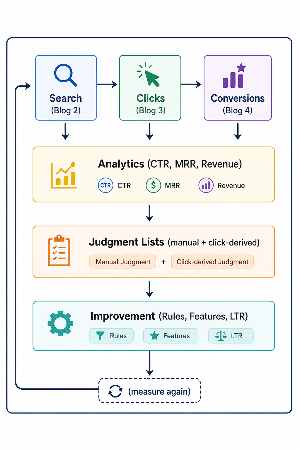
The key insight is that the same instrumentation that measures search quality also generates the data to improve it. Your search spans produce the queries to analyze, and your click spans produce the judgment data for evaluation and LTR training. Plus, your conversion spans tell you which improvements matter most to the business.

Measuring search relevance improvements after changes

After deploying a change, like a new query rule or updated field weights, or deploying an LTR model, you need to know whether it helped:

Run the same ES|QL queries before and after. If your change was a query rule for "laptop bag", compare that query's CTR and MRR from the week before to the week after.

A/B testing with experiment attributes

The feature_flag.key attribute  is designed for exactly this. Route a percentage of traffic to a new ranking configuration, and set feature_flag.key to the experiment name and optionally feature_flag.result.variant to the variant (for example, "control" or "variant-boost-v2"). Then propagate it to click spans the same way you propagate `query_id`, and compare metrics between groups:

FROM traces-generic.otel-default
| WHERE ((name == "search" AND attributes.search.query IS NOT NULL)
    OR attributes.search.first_click == true)
  AND attributes.feature_flag.key IS NOT NULL
| STATS
    searches = COUNT(CASE(name == "search" AND attributes.search.query IS NOT NULL, 1)),
    clicked = COUNT(CASE(attributes.search.first_click == true, 1))
  BY attributes.feature_flag.key, attributes.feature_flag.result.variant
| EVAL ctr_pct = ROUND(100.0 * clicked / searches, 1)

This gives you an A/B comparison of CTR by experiment variant. You don’t need a separate experimentation platform for basic comparisons, although you’ll want a proper framework for statistical rigor on sample sizes and significance.

Monitoring for search relevance regressions

Once you've identified your high-value queries, that is, the ones that drive revenue and have been tuned for good engagement, you need to protect them. Relevance regressions on your top 20 revenue-generating queries are business-critical incidents.

This is where monitoring comes in. In the next blog in the series, we'll cover setting up alerts on these metrics: CTR drops on high-revenue queries and MRR regressions after deployments. We’ll also cover conversion rate anomalies. The same ES|QL queries that power your analytics dashboards can drive alerting rules; the feedback loop covers measurement and improvement. It also provides operational protection.

Search relevance improvement roadmap: Week 1 to Quarter 1

Here's a practical starting point. You don't need to implement LTR on day one. The approaches build on each other:

• Week 1: Evaluate and fix known problems. Run the CTR-by-query analysis. Find your zero-CTR queries with high search volume, and fix the worst ones with synonyms or pinned results via query rules. You could also use adjusted field weights. Use judgment lists (even a small manual one for your top queries) to confirm that the changes improve NDCG before deploying. You should get immediate, targeted impact.

• Month 1: Add behavioral rank features. Extract document-level click popularity and conversion rates from your analytics. Index them as rank_feature fields, and blend behavioral signals with text relevance using the linear retriever or `rank_feature` queries. Then consider simple business boosts like margin. This lifts baseline quality across all queries without manual intervention per query.

• Quarter 1: Automate with LTR. Once you have enough click data (typically several weeks of production traffic), build judgment lists automatically from click and conversion data. Train an LTR model that combines text features, behavioral features, and business features, and then deploy it as a rescorer. The ranking now learns from user behavior and improves as you collect more data.

At each stage, measure the impact with the same metrics. CTR and MRR are your scorecards, as is conversion rate. If a change doesn't move them, it didn't help, regardless of how sophisticated the approach.

What's next: Search reliability engineering and SLOs

We've covered the full sequence: instrument search, measure quality, track conversions, and improve relevance. The missing piece is making sure it all keeps working.

Next, we close the series with search reliability engineering, including Service Level Objectives (SLOs) for search quality and alerting on metric regressions, along with operational dashboards that catch problems before users notice them. The same metrics you've been building become the basis for search health monitoring, turning your analytics pipeline into a reliability system.

Get started

Working code

• Reference project: Working code for the entire blog series; clone, configure, and run.