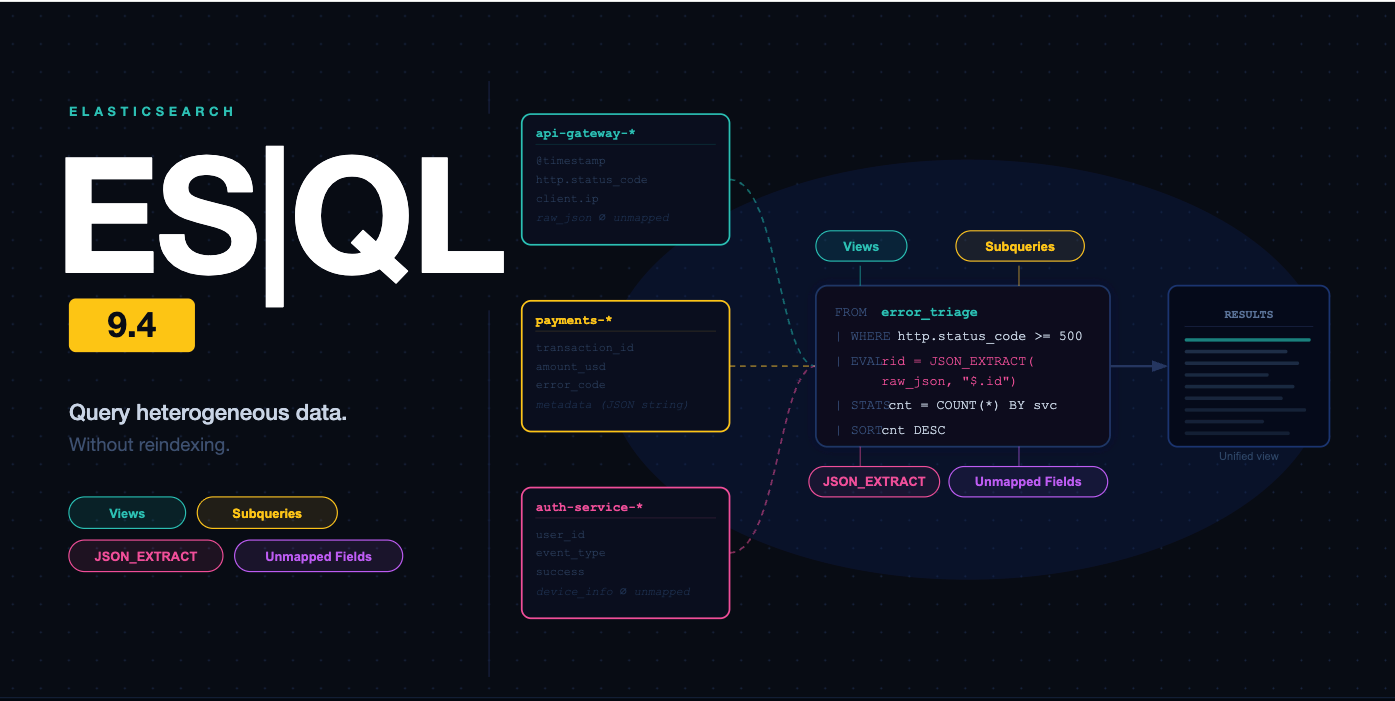
From Elasticsearch runtime fields to ES|QL: Adapting legacy tools to current techniques

Elasticsearch runtime fields solve the problem of computing values at query time without reindexing. But they come with Painless scripting complexity and performance costs that scale with document count. Elasticsearch Query Language (ES|QL) offers a more powerful alternative with a dedicated execution engine, pipeline processing, and no scripting required. In this article, you’ll learn how to map five common runtime field patterns to their ES|QL equivalents, so you can modernize your queries and understand when each approach makes sense.

Prerequisites

• Elasticsearch 8.15+ (for :: cast operator support; core ES|QL features available from 8.11)

Runtime fields versus ES|QL

Runtime fields were introduced in Elasticsearch 7.11 as a way to define fields at query time. Instead of reindexing data, you could write a Painless script that computes values on the fly:

PUT my-index/_mapping
{
  "runtime": {
    "full_address": {
      "type": "keyword",
      "script": {
        "source": "emit(doc['address'].value + ':' + doc['port'].value)"
      }
    }
  }
}

This works, but comes with trade-offs:

• Painless scripting overhead: Every runtime field requires scripting knowledge, and the syntax is Java-like, not query-like.

• Performance cost: Runtime fields evaluate per document at query time. Elasticsearch classifies them as "expensive queries" that can be rejected by cluster settings.

• Isolated computation: Each runtime field computes independently. There’s no way to chain transforms or use the output of one field in another within the same query.

ES|QL changes the equation. It has its own execution engine (not translated to Query DSL), runs queries concurrently across nodes, and provides a complete toolkit for field computation: EVAL, GROK, DISSECT, type casting, and pipeline chaining.

Let's see how each runtime field pattern maps to ES|QL.

Setting up the example data

All the code snippets in this article can be executed in the Kibana Dev Tools console.

To follow along, create a sample index with data that exercises all five patterns. This simulates a server logs scenario with mixed field types, raw messages, and some intentional data quality issues:

PUT server-logs
{
  "mappings": {
    "properties": {
      "host": { "type": "keyword" },
      "port": { "type": "keyword" },
      "raw_message": { "type": "text" },
      "response_time": { "type": "keyword" },
      "status_code": { "type": "keyword" },
      "region": { "type": "keyword" }
    }
  }
}

Now index some sample documents:

POST _bulk
{ "index": { "_index": "server-logs" } }
{ "host": "web-01", "port": "8080", "raw_message": "2024-01-15 INFO user=alice action=login duration=230ms", "response_time": "145", "status_code": "200", "region": "us-east" }
{ "index": { "_index": "server-logs" } }
{ "host": "web-02", "port": "443", "raw_message": "2024-01-15 ERROR user=bob action=upload duration=1200ms", "response_time": "not_available", "status_code": "500", "region": "eu-west" }
{ "index": { "_index": "server-logs" } }
{ "host": "api-01", "port": "3000", "raw_message": "2024-01-15 WARN user=charlie action=query duration=890ms", "response_time": "890", "status_code": "200", "region": "us-east" }
{ "index": { "_index": "server-logs" } }
{ "host": "api-02", "port": "3000", "raw_message": "2024-01-16 INFO user=diana action=export duration=3400ms", "response_time": "3400", "status_code": "200", "region": "ap-south" }
{ "index": { "_index": "server-logs" } }
{ "host": "web-01", "port": "8080", "raw_message": "2024-01-16 ERROR user=eve action=login duration=50ms", "response_time": "50", "status_code": "401", "region": "US-EAST" }

Notice that response_time is stored as a keyword (a common real-world mistake), and the last document has "US-EAST" instead of "us-east" (a data quality issue we’ll fix later).

Pattern 1: Field concatenation

A common runtime field use case is combining two fields into one. For example, creating a host:port identifier.

The runtime field approach

You can define it inline at query time. Query-time approach avoids modifying the mapping, but you still need Painless scripting, scoping it to a single search request:

GET server-logs/_search
{
  "runtime_mappings": {
    "endpoint": {
      "type": "keyword",
      "script": {
        "source": "emit(doc['host'].value + ':' + doc['port'].value)"
      }
    }
  },
  "fields": ["endpoint"],
  "_source": false
}

The ES|QL approach

You can run ES|QL queries using the _query API endpoint:

POST _query
{
  "query": """
    FROM server-logs
    | EVAL endpoint = CONCAT(host, ":", port)
    | KEEP host, port, endpoint
    | LIMIT 1
  """
}

Response:

{
  "columns": [
    { "name": "host", "type": "keyword" },
    { "name": "port", "type": "keyword" },
    { "name": "endpoint", "type": "keyword" }
  ],
  "values": [
    ["web-01", "8080", "web-01:8080"]
  ]
}

CONCAT accepts two or more arguments and always returns a keyword.

Note: For brevity, the remaining ES|QL examples in this article show just the query. Wrap them in POST _query { "query": "..." } to run them in Kibana Dev Tools.

When to use

If you need endpoint to persist across all queries and be available in Kibana dashboards, use a mapping-level runtime field. If you need it for a single search request within Query DSL, use a query-time runtime field. If you need it for ad-hoc analysis or exploratory work, ES|QL is simpler.

Pattern 2: Data extraction from unstructured text

Extracting structured data from raw log messages is another classic runtime field pattern.

The runtime field approach

Painless uses Java's regex Matcher class:

GET server-logs/_search
{
  "runtime_mappings": {
    "log_user": {
      "type": "keyword",
      "script": {
        "source": "def matcher = /user=(\\w+)/.matcher(params._source['raw_message']); if (matcher.find()) { emit(matcher.group(1)); }"
      }
    }
  },
  "fields": ["log_user"],
  "_source": false
}

This is verbose. You need to know Painless regex syntax, handle the Matcher object, and call emit() correctly.

The ES|QL approach: GROK

ES|QL provides two purpose-built commands for text extraction. GROK uses regex-based patterns:

FROM server-logs
| GROK raw_message "%{WORD:timestamp_date} %{WORD:log_level} user=%{WORD:user} action=%{WORD:action} duration=%{WORD:duration}"
| KEEP user, log_level, action, duration

Response:

{
  "columns": [
    { "name": "user", "type": "keyword" },
    { "name": "log_level", "type": "keyword" },
    { "name": "action", "type": "keyword" },
    { "name": "duration", "type": "keyword" }
  ],
  "values": [
    ["alice", "INFO", "login", "230ms"], ...
  ]
}

GROK uses the %{SYNTAX:SEMANTIC} pattern format. It extracts multiple fields in a single and readable command.

The ES|QL approach: DISSECT

For structured data with consistent delimiters, DISSECT is faster because it doesn’t use regular expressions:

FROM server-logs
| DISSECT raw_message "%{timestamp_date} %{log_level} user=%{user} action=%{action} duration=%{duration}"
| KEEP user, log_level, action, duration

The syntax is nearly identical to GROK, but DISSECT works by splitting on delimiters rather than matching regex patterns. This makes it faster for data that follows a consistent format.

When to use GROK vs DISSECT

Use DISSECT when your data has a predictable structure (same delimiters, same field order). Use GROK when you need regex flexibility, for example when fields may be optional or formats vary.

Pattern 3: Dynamic type conversion

When a field is mapped as keyword but contains numeric data (a surprisingly common scenario), runtime fields can cast it at query time.

The runtime field approach

GET server-logs/_search
{
  "runtime_mappings": {
    "response_time_long": {
      "type": "long",
      "script": {
        "source": """
          def val = doc['response_time'].value;
          if (val != 'not_available') {
            emit(Long.parseLong(val));
          }
        """
      }
    }
  },
  "fields": ["response_time_long"],
  "_source": false
}

You need to handle parsing exceptions manually. If Long.parseLong fails on an unexpected value, the script throws an error.

The ES|QL approach

ES|QL provides explicit conversion functions and a shorthand cast operator:

FROM server-logs
| EVAL response_ms = TO_LONG(response_time)
| KEEP host, response_time, response_ms

Or with the :: cast operator (available since 8.15):

FROM server-logs
| EVAL response_ms = response_time::long
| KEEP host, response_time, response_ms

Response:

{
  "columns": [
    { "name": "host", "type": "keyword" },
    { "name": "response_time", "type": "keyword" },
    { "name": "response_ms", "type": "long" }
  ],
  "values": [
    ["web-01", "145", 145]
  ]
}

Both produce the same result. The key difference from Painless: Failed conversions return null instead of throwing exceptions. The document with "not_available" simply gets null for response_ms, and ES|QL emits a warning.

Common conversion functions include:

The :: operator works with all these types (for example, field::double, field::datetime).

When to use

ES|QL's graceful null handling makes it safer for dirty data. Runtime fields with Painless give you fine-grained control over error handling but require more code. For type conversion specifically, ES|QL is almost always the better choice.

Pattern 4: Dynamic field handling

Runtime fields support "dynamic": "runtime" in mappings, which prevents mapping explosion by creating all new fields as runtime fields instead of indexed fields:

{
  "mappings": {
    "dynamic": "runtime",
    "properties": {
      "timestamp": { "type": "date" }
    }
  }
}

Any new field sent to this index becomes a runtime field automatically. This is useful when you ingest semi-structured data with unpredictable field names.

Where ES|QL fits

ES|QL provides query-time flexibility, but it still needs fields to be visible in the mapping. This is where runtime fields and ES|QL complement each other rather than compete.

If a field exists in _source but isn’t mapped, ES|QL cannot access it directly. The current workaround is to define a runtime field to make the unmapped field visible:

PUT dynamic-logs/_mapping
{
  "runtime": {
    "custom_field": {
      "type": "keyword",
      "script": {
        "source": "emit(params._source['custom_field'])"
      }
    }
  }
}

Once defined, ES|QL can query it:

FROM dynamic-logs
| WHERE custom_field == "some_value"
| KEEP timestamp, custom_field

This is one scenario where runtime fields remain essential. They act as a bridge, making unmapped data accessible to ES|QL.

Pattern 5: Field shadowing for error correction

Runtime fields can shadow (override) indexed fields by defining a runtime field with the same name as an existing field. This is useful for correcting data without reindexing.

The runtime field approach

Remember our data quality issue, where region has inconsistent casing ("US-EAST" versus "us-east")?

GET server-logs/_search
{
  "runtime_mappings": {
    "region": {
      "type": "keyword",
      "script": {
        "source": "emit(params._source['region'].toLowerCase())"
      }
    }
  },
  "fields": ["region"],
  "_source": false
}

This overrides the indexed region field for all queries. Every search, aggregation, and Kibana visualization will see the lowercase version.

FROM server-logs
| EVAL region = TO_LOWER(region)
| KEEP host, port, region

When you use EVAL with an existing column name, ES|QL drops the original column and replaces it with the computed value. This is the exact equivalent of field shadowing, but scoped to the current query.

You can also chain multiple corrections in a pipeline:

FROM server-logs
| EVAL region = TO_LOWER(region)
| EVAL region = CASE(region == "us-east", "US East", region == "eu-west", "EU West", region == "ap-south", "AP South", region)
| KEEP host, region

When to use

If the correction should apply to all queries and Kibana dashboards, use runtime field shadowing. If you need to correct data for a specific analysis, ES|QL is more flexible since you can apply different transformations in different queries without modifying the mapping.

The ES|QL pipeline advantage: Going beyond runtime fields

This is where ES|QL fundamentally surpasses runtime fields. Runtime fields are isolated: each one computes independently, and you cannot use the output of one runtime field as input for another in the same query.

ES|QL pipelines chain transforms. Here’s a single query that combines multiple patterns:

FROM server-logs
| GROK raw_message "%{WORD:log_date} %{WORD:log_level} user=%{WORD:user} action=%{WORD:action} duration=%{INT:duration_raw}ms"
| EVAL duration_ms = duration_raw::long
| EVAL region = TO_LOWER(region)
| WHERE log_level == "ERROR" AND duration_ms > 100
| STATS avg_duration = AVG(duration_ms), error_count = COUNT(*) BY region

This single query:

• Extracts fields from raw text (GROK).

• Converts the duration to a number (EVAL with cast).

• Normalizes region casing (EVAL with TO_LOWER).

• Filters for errors with high duration (WHERE).

• Aggregates by region (STATS).

To achieve the same result with runtime fields, you would need to define at least three separate runtime fields (for extraction, conversion, and normalization) and then write a Query DSL query with filters and aggregations. The ES|QL version is a single, readable pipeline.

You can even use expressions directly inside aggregations:

FROM server-logs
| EVAL response_ms = response_time::long
| STATS
    avg_response = AVG(response_ms),
    p95_response = PERCENTILE(response_ms, 95),
    slow_count = COUNT(CASE(response_ms > 1000, 1, null))
  BY host

Conclusion

What we covered:

• ES|QL provides a full toolkit (EVAL, GROK, DISSECT, type casting with ::) that replaces most runtime field patterns without any Painless scripting.

• Failed type conversions in ES|QL return null instead of throwing exceptions, making it safer for real-world data.

• Pipeline processing (chaining GROK into EVAL into WHERE into STATS) goes beyond what runtime fields can do in isolation.

• Runtime fields remain valuable for persistent computed fields, field shadowing across all queries, and as a bridge for unmapped data in ES|QL.

One important caveat: Both runtime fields and ES|QL compute values at query time, which means they pay the cost on every query. If you find yourself applying the same transformation repeatedly (type corrections, field extraction, data normalization), consider using ingest pipelines to fix the data at index time instead. Ingest pipelines let you parse, enrich, and transform documents before they’re stored, so queries can work with clean, properly typed fields directly. Runtime fields and ES|QL are great for exploration and ad-hoc analysis, but for production workloads, indexing the right data from the start is almost always the better choice.

The key takeaway: Runtime fields aren’t deprecated, and they aren’t going away. But for most query-time computation patterns, ES|QL offers a simpler, more powerful, and more performant approach. And when the transformation is known up front, an ingest pipeline is the most efficient option of all.

Next steps

• ES|QL documentation

• Runtime fields reference

• ES|QL timeline of improvements

• Getting started with runtime fields

• ES|QL processing data with DISSECT and GROK