Elasticsearch, Kibana, Elastic Cloud 8.4: Reduce size for metric data


 Share on Twitter
Share on Twitter

 Share on LinkedIn
Share on LinkedIn

 Share on Facebook
Share on Facebook

 Share by Email
Share by Email

 Print this page
Print
We are pleased to announce the release of Elastic 8.4.
In Elasticsearch, synthetic _source is the first of many future innovations designed to reduce storage for machine generated data. An impressive reduction in index size by tens of percentage points will help you store more metric data at the same cost. Elasticsearch also welcomes KNN to the _search API endpoint. You can now implement similarity search on vector embeddings directly from the _search syntax you are familiar with.
Analyze and reduce MTTR of production problems or security threats with the “explain log rate spikes” functionality. Using explain log rate spikes, you can easily identify the root cause of significant deviations in your log message rates.
Finally in 8.4, Kibana introduces a new option for scheduling snoozes for alerts which can help you filter out unnecessary noise by temporarily suppressing notifications due to known or planned environment disruptions.
Ready to roll up your sleeves and get started? We have the links you need:
- Start Elasticsearch on Elastic Cloud
- Download Elasticsearch, Kibana, Integrations
- 8.4 Release notes for Elasticsearch, Kibana
- 8.4 Breaking changes
Synthetic _source, accelerating ways to analyze all your machine generated data in one place
At Elastic, we continue to optimize our Elastic Observability solution and the storing of o11y data sources like logs, metrics, and traces. These optimizations not only improve o11y use case but can be applied to our security solution built and stored on a single data store, Elasticsearch.
In 8.4, we are releasing a new feature called synthetic _source. This option significantly reduces the index size, which can be used with machine generated data like logs and metrics. Synthetic _source is one feature in a series of enhancements we are planning to release for optimizing time-series data such as metrics on Elasticsearch. Subsequent phases will include improving the ability to analyze the delta of a metric in a time series as a function of time (e.g., rate on counter that handles resets, sliding weekly average, and speed/direction in asset tracking), further reduction in index size, and downsampling as an Index Lifecycle Management (ILM) action.
When Elasticsearch ingests documents, it saves them in a number of data structures, each optimized for particular types of usage. One of these data structures is called _source, and it simply holds the fields of the document exactly like when Elasticsearch received them. _source is used in various places, including reindexing and presenting the document in Kibana Discover. The problem with _source is that it takes a lot of space.
With synthetic _source Elasticsearch recreates the _source when needed from doc_values. doc_values is our columnar repository, used for aggregation, sorting, and access by scripts, so in practice, the data in the field is almost always saved also to doc_values. We thought, why save it twice if we can keep only one and recreate the other when needed?
With synthetic _source, Elasticsearch re-hydrates the _source from doc_values saving a significant amount of space on the index. The performance of _source retrieval may be a bit different when compared to saving _source in a separate structure, as it may take a few extra milliseconds to recreate _source from doc_values, but on other occasions it will be faster than retrieving it directly from _source. In any case, the retrieval performance impact in either direction was minor in all the tests we conducted.
Using synthetic _source significantly improves the performance of indexing data into Elasticsearch because there is no need to write to the _source data structure. Faster indexing is great, but it pales in comparison to the overall reduction in index size in the multiples of 10 percent! We are excited about this new change in storing and analyzing metric data. In the future, we look forward to delivering metrics-specific functionality that will drive out goal for Elasticsearch becoming the next generation complete time-series data platform.
In 8.4, Synthetic _source is in technical preview and only supports a subset of the data types. If you refer in the documentation, the commonly used data types in machine generated data are fully supported.
Scalable vector search with hybrid scoring in the _search API endpoint
In many scenarios, the best relevance ranking uses multiple indicators, rather than a single one. For example, if the data and queries include texts and images, the images may be best ranked by vector similarity while the text may be best ranked by BM25F, and ultimately the documents should be sorted by a combination of both scores. The same is true when analyzing only text —e.g., depending on the documents and queries, both BM25F (perhaps with other indicators, like popularity) and vector similarity could contribute to the overall ranking. Oftentimes the decision regarding the importance of the vector similarity score versus the importance of the BM25F score can only be determined after analyzing the specific query.
In 8.4, we enable support for a hybrid scoring, using a linear combination of vector similarity and traditional ranking methods, such as BM25F. The search request accepts a weight for each of the components, and the documents are ranked by the weighted sum of the two scores. The big benefit of linear combination for hybrid search is that it is very easy to understand and use it, so we opted to start with the simplest way, allowing users to invest their effort in analyzing the queries and scenarios coming up with the best weights. In the future, we will consider support for other hybrid combination methods that allow the result sets to be combined in more nuanced ways.
In 8.2, we introduced the ability to filter with KNN vector search. This was quite complex to achieve, but also very useful, because it allows users to use facets to add context to their search and eliminate false positives. The question still remained: how do you choose the values that the user will be able to filter by (i.e., the facet values)?
In traditional search (e.g., BM25F based), there is an inherent filter: if the terms in the query are not included in the document, the document will not be in the result set. That filter allows aggregating the values from the documents in the result set to generate the facet values. In vector similarity, this is quite different, since even the most irrelevant document in the index has some similarity (e.g., some dot product, with the vector of the query). In 8.4 we opted to enable aggregations on the k most similar documents in the result set, so users get the power of Elasticsearch aggregations and can provide the most relevant filtering options as facets to end users.
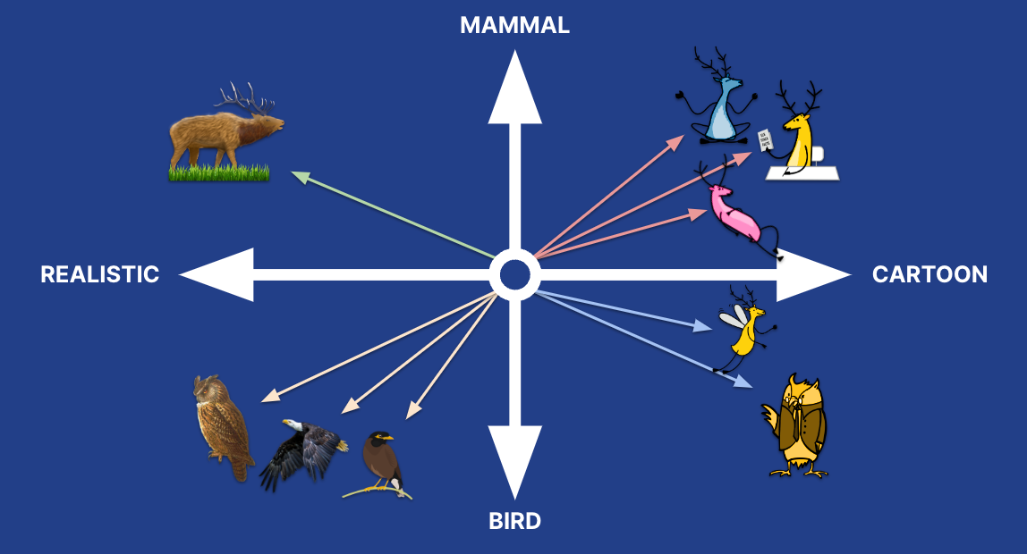
In the oversimplified model above, even the realistic birds have some cosine similarity to the yellow cartoon elk, even though they are the furthest from it in terms of vector similarity. If we were to filter the result set by color, we would probably want the filter options to have pink and blue, based on the values of the more relevant results, rather than black, which would bring results that are really irrelevant. For that reason, we opt to aggregate on the top k results rather than on all the results.
Now that you can use kNN search with functionality like filtering, aggregations, hybrid search, and more, we decided to add the kNN vector search to the _search API. In 8.0, when we introduced the _knn_search API, we exposed the capabilities temporarily so users could experiment and provide feedback. We got a lot of feedback including the adding kNN vector search to the _search API. For us, this is one of the final phases before turning kNN vector search from technical preview to generally available.
Explain log rate spikes
As a step toward automatically analyzing the root cause of potential observability issues or security threats, the “Explain log rate spikes” feature is available in the Machine Learning app under AIOps in 8.4. Explain log rate spikes identifies statistically significant deviations from the baseline log rate and which fields contribute the most to the deviation, thus delivering an initial explanation that’s a good starting point for drilling deeper into root causes. This is currently in tech preview and complements our standard anomaly detection that’s already available in Kibana.
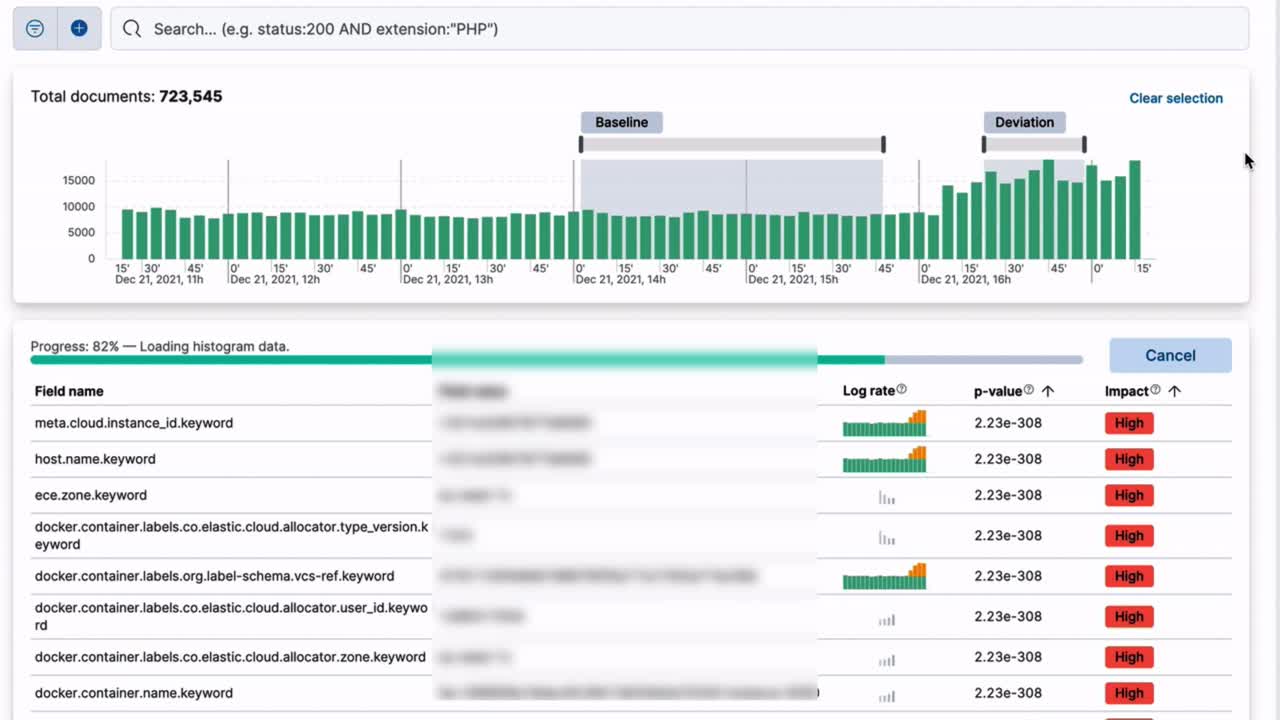
Log spike analysis enables you to identify reasons of log rate increase even in millions of logs across multiple fields and values. The histogram makes it easy to find spikes in log rates, and the intuitive user interface enables you to compare the deviation to a baseline. The analysis shows the fields and their values that have the biggest impact on the message rate deviation.
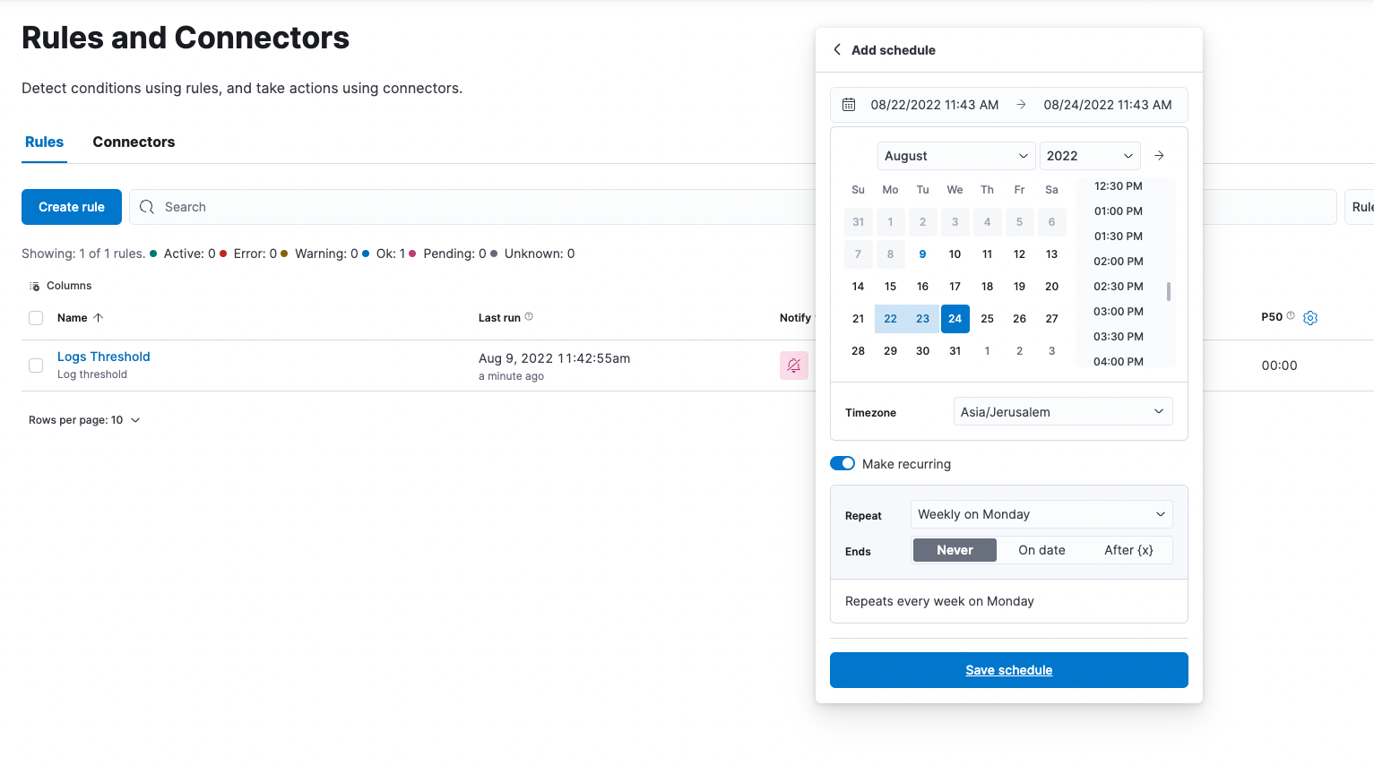
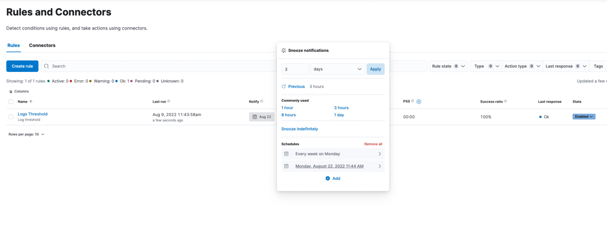
Scheduled snooze for your alerting rules
Sometimes you know you’re about to make a disruptive change and you need to preemptively (and temporarily) disable specific alert rules to prevent an unnecessary fire drill for your team. Other times, you may already be resolving an already-firing alert rule and want to prevent future execution of that rule from distracting the team as the alert has already been assigned. In 8.4, we are bringing a snooze option to alert rules, allowing you to temporarily suppress notifications. Learn more about managing alerting rules in Kibana docs.
Vector tiles used for geo retrieval just got even faster!
When we introduced vector tiles into Elasticsearch in 7.15, they provided massive improvement in both scalability and performance when presenting geographic data on a map. Our experience is that when we introduce such a significant technological leap, we later find ways to further optimize it in Lucene. It is not an easy task, but with a lot of smart engineering, and a deep understanding of the underlying mechanism, we were able to make a very significant optimization to vector tiles in 8.4.
When computing the projection from WGS84 (a cartography and geodesy standard) to spherical mercator, we opted for using sloppy math instead of the exact math we currently were using. This change reduced query latency and the required computing resources significantly, in particular when used on big geometries. The beauty is that in this specific case, the extent of the sloppiness is anyway not represented in the final result you get (the result is more accurate than can be presented), so we get all the benefits of the sloppy math, without any downside.
If that was all too theoretical or technical, here’s the bottom line: 5% to 10% reduction in vector tiles query latency! That maps directly to lower costs and better user experience.
Transforms : Infinite and adaptive retries
With the increasing adoption of transforms, it has become more important for them to run unattended. It is better that a transform recovers without any user intervention after a problem with the cluster is fixed rather than for a user to have to manually restart it.
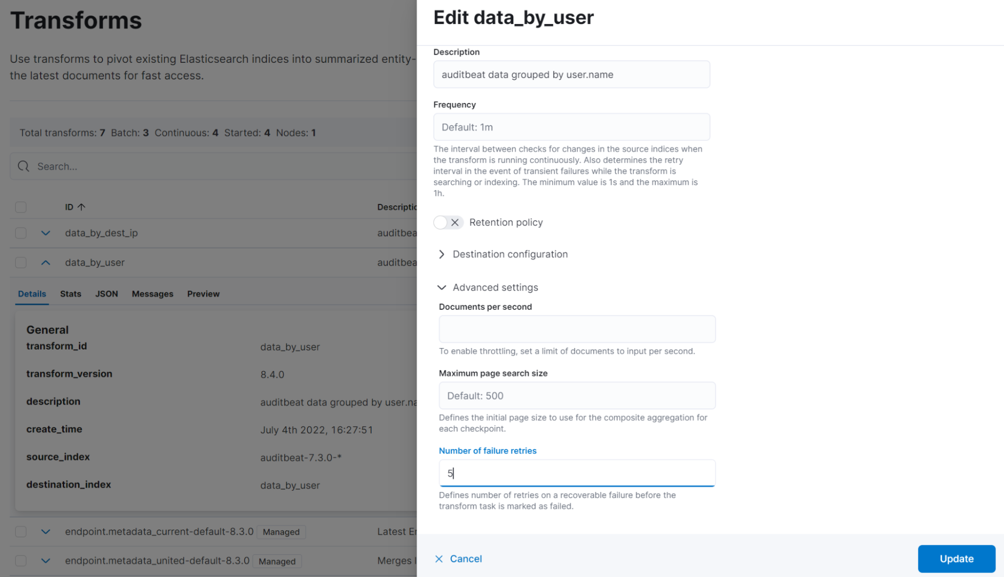
Infinite and adaptive retries — available in 8.4 — make it possible for transforms to recover after a failure without any user intervention. The transform retries will back off progressively, and retries can be configured per transform. The interval between retries doubles after reaching a one-hour threshold. This is because the possibility that retries solve the problem is less likely after each failed retry.
In the transforms page in Kibana Stack Management, the number of retries can be configured when creating a new transform or editing an existing one. If not set, the cluster setting xpack.transform.num_transform_failure_retries, or a default of 10, will be used. Unlimited retries can be achieved by setting the number of retries to -1.
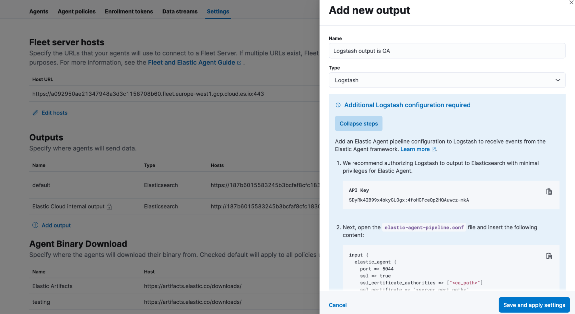
Fleet managed agent output to Logstash is now GA
Back in 8.2, we announced the support for agent output to Logstash as beta and have seen great adoption and feedback on the UX and usability. And with this release, we feel confident in announcing general availability of Logstash output support for fleet managed agent as generally available (GA).
Customize ingest pipelines, templates of built-in integrations!
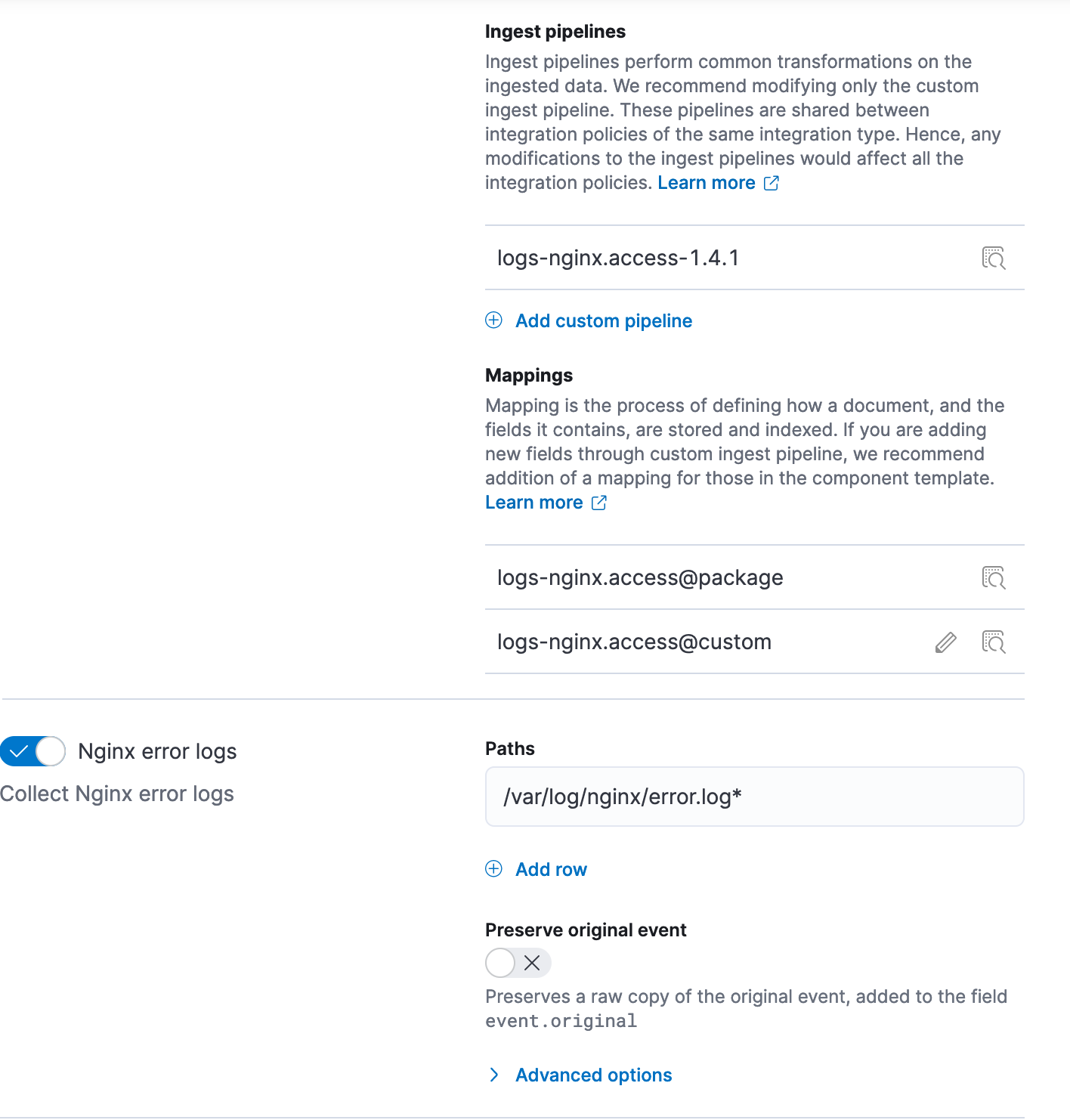
Built-in fleet integrations contain all the required data plumbing, such as index templates, settings, and mappings for the datastream where the integration data is to be stored, for enabling out of the box experience observability and security solutions. However, you may need to update this plumbing for use cases such as enriching with additional fields to the integration data, dropping unnecessary data, redacting confidential data, adding computed fields such as timezones to timestamps, etc.
Today, users can achieve these outcomes for an existing integration by modifying the ingest pipeline; however, their changes are overwritten whenever the integration is upgraded. We are pleased to announce that you can customize the integration’s ingest pipelines and mappings, right from the integration UI, your one place to manage lifecycle of integrations with Elastic.
In addition to built-in integrations which come with ingest pipelines, this functionality will also improve experience of defining data plumbing for use cases where you are using our integrations such as custom logs to just collect logs and are defining your own data transformation with your own ingest pipeline and mapping.
Try it out
Existing Elastic Cloud customers can access many of these features directly from the Elastic Cloud console. If you’re new to Elastic Cloud, take a look at our Quick Start guides (bite-sized training videos to get you started quickly) or our free fundamentals training courses. You can always get started for free with a free 14-day trial of Elastic Cloud or download the self-managed version of the Elastic Stack for free. Or get started today by signing up via AWS Marketplace, Google Cloud Marketplace, or Microsoft Azure Marketplace.
Read about these capabilities and more in the release notes, and other Elastic Stack highlights in the Elastic 8.4 announcement post.
The release and timing of any features or functionality described in this post remain at Elastic's sole discretion. Any features or functionality not currently available may not be delivered on time or at all.
Share
- Share on Twitter
Share on Twitter
- Share on LinkedIn
Share on LinkedIn
- Share on Facebook
Share on Facebook
- Share by Email
Share by Email
- Print this page
Print