Machine learning in cybersecurity: Training supervised models to detect DGA activity
How annoying is it when you get a telemarketing call from a random phone number? Even if you block it, it won’t make a difference because the next one will be from a brand new number. Cyber attackers employ the same dirty tricks. Using domain generated algorithms (DGA), malware creators change the source of their command and control infrastructure, evading detection and frustrating security analysts trying to block their activity.
In this two-part series, we’ll use Elastic machine learning to build and evaluate a model for detecting domain generation algorithms. Here in part 1, we’ll cover:
- The process of extracting features from the raw malicious and benign domains
- Explain a bit about the process of finding suitable features
- Show you how to train and evaluate a machine learning model using the Elastic Stack
In part 2, we’ll discuss how to deploy the trained model into an ingest pipeline to enrich Packetbeat data at ingest time. Configuration files and supporting materials will be available in the examples repository.
If you’d like to try this out at home, I’d recommend spinning up a free trial of our Elasticsearch Service, where you’ll have full access to all of our machine learning capabilities. Ok, let’s dive into it.
DGA: A background
After infecting a target machine, many malicious programs attempt to contact a remote server — a so-called command & control (C&C or C2) server — to exfiltrate data and receive instructions or updates. This means that the malicious binary has to either know the IP address of the C&C server, or the domain. If this IP address or domain is hardcoded into the binary, it is relatively easy for defensive measures to thwart this communication by adding the domain to a blocklist.
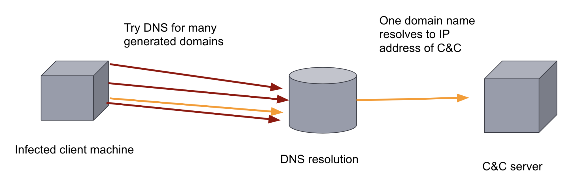
To subvert this defensive measure, malware authors can add a DGA to their malware. DGAs generate hundreds or thousands of random-looking domains. The malware binary on the infected machine then cycles through each of the generated domains, trying to resolve the domain names to see which one of the domains has been registered as the C&C server. The sheer volume and randomness of the domains makes it hard for a rule-based defensive approach to thwart this communication channel. It also makes it hard for a human analyst to find since DNS traffic is usually very high-volume. Both of these factors make it an ideal application of machine learning.
Training a machine learning model to classify domains
In supervised machine learning, we provide a labeled training dataset of malicious and benign domains, allowing a model to learn from that dataset so that it can then be used to classify previously unseen domains as either malicious or benign.
There are various different types of DGAs — not all of them look the same. Some DGAs produce random looking domains, others use word-lists. For production models, different features and models can be used to capture the characteristics of the different algorithms. In this example we will train a single model based on the characteristics found in the most common algorithms.
Here we are going to use a dataset composed of domains from various malware families and benign domains to train our model.
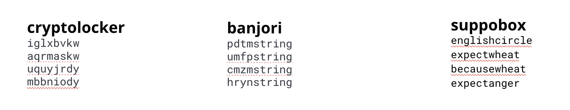
cryptolocker, banjori and suppobox malware families
Feature engineering
The input required to create an effective machine learning model are features that can capture the characteristics of the domains generated by DGAs. We therefore have to tell the model which aspects of the string are important for distinguishing between malicious and benign domains. This is known as feature engineering in the world of machine learning.
Understanding the features that best distinguish benign from malicious domains is an iterative process. For example, we started with some simple features like domain name length and domain name entropy, but the resulting models were not particularly accurate compared to other methods such as the LSTM. These models take advantage of the sequential characteristics of the strings, so we then looked at other features which would encode sequences more effectively.
After iterating through several feature engineering approaches, we concluded that using the presence of substrings of various lengths would best capture the difference between malicious and benign domains in the model.
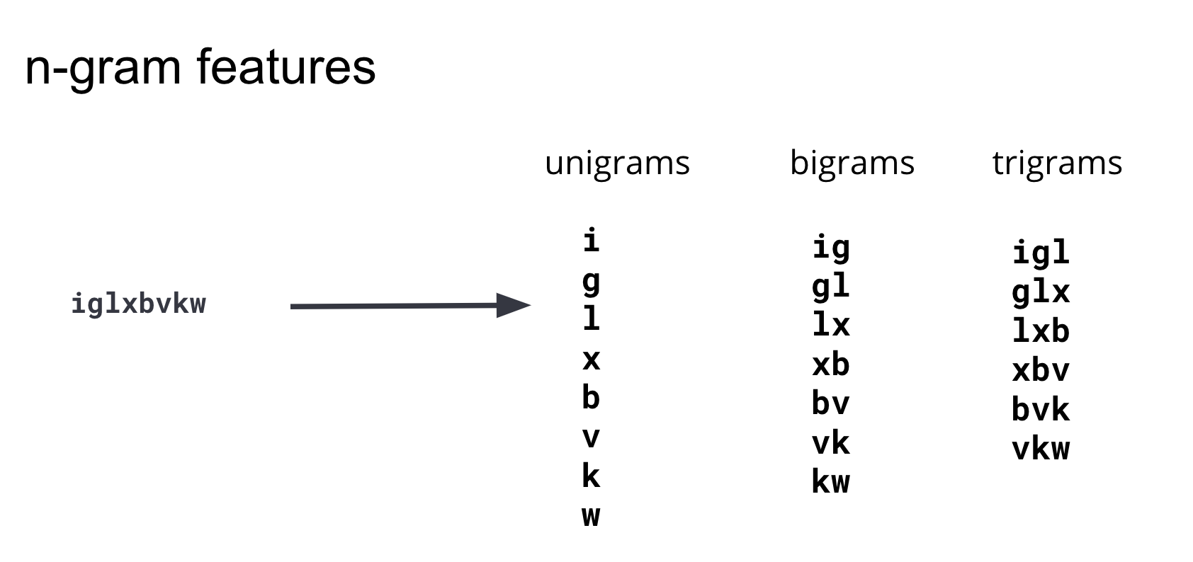
These substrings are commonly known as n-grams. When developing features, it’s important to balance the number of features (the dimensionality of the training dataset) and the complexity of computing the features with their benefit to the model. After iterating and testing n-grams of various lengths, we concluded that n-grams with length 4 or longer did not add significant predictive information to the model and thus our feature set is restricted to unigrams, bigrams and trigrams. The diagram in Figure 3. illustrates how these features are generated from an example domain.
To generate an Elasticsearch index that has each DGA domain split into unigrams, bigram and trigrams, you can re-index the original source index through an ingest pipeline with a painless script processor. An example is shown in Figure 4 below. For full configurations, instructions, and various customization options, please refer to the examples repository.
POST _scripts/ngram-extractor-reindex
{
  "script": {
    "lang": "painless",
    "source": """
      String nGramAtPosition(String fulldomain, int fieldcount , int n){
        String domain = fulldomain.splitOnToken('.')[0];
        if (fieldcount+n>=domain.length()){
          return ''
        }
        else
        {
          return domain.substring(fieldcount, fieldcount+n)
        }
      }
      for (int i=0;i<ctx['domain'].length();i++){
        ctx[Integer.toString(params.ngram_count)+'-gram_field'+Integer.toString(i)] = nGramAtPosition(ctx['domain'], i, params.ngram_count)
      }
    """
  }
}
Normally, one would need to do more pre-processing to convert the substrings of lengths 1, 2, and 3 into numerical vectors for the machine learning algorithm. In our case, Elastic machine learning will take care of this conversion to numerical values, otherwise known as encoding. Elastic machine learning will also examine the features and automatically select those that carry the most information.
Creating a Data Frames Analytics job
The next step is to use the Data Frame Analytics UI to create a classification job. I’ve highlighted some important aspects of this process in the screenshots below.
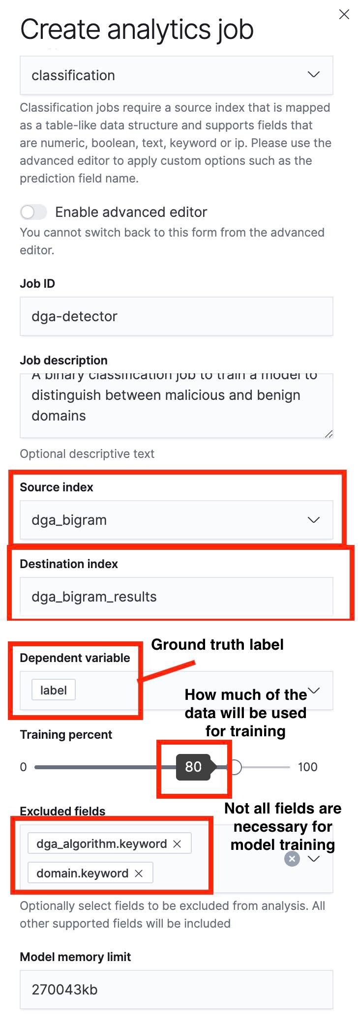
A key thing to notice is that we can specify a train/test split using the slider. In the screenshot in Figure 5, the train/test split is set to 80%, which means that 80% of the documents in the source index will be used for training the model and the remaining 20% will be used for testing the model.
Once the training process has completed, we can navigate to the Data Frame Analytics Results UI to evaluate the performance of the model. Since we split our source index into a training set and a test set, we will be able to see the model’s performance on each. While both training performance and test performance provide valuable information, in this case we will be more interested in the performance of the model on the test dataset, as it will give us an idea of the generalization error in a model. This error indicates how the model will perform on data points it has not encountered before.
Evaluating a machine learning model
Once the training process is complete, we can click through to “View” the results from the Elastic machine learning UI job management page.
The results page (see Figure 6) gives us two key pieces of information: a confusion matrix that summarizes how our model has performed and a table of results where we can drill down to view how individual data points were classified by the model. We can toggle between the confusion matrix and summary table for the testing and training datasets by using the Testing/Training filters on the top right hand side of the table.
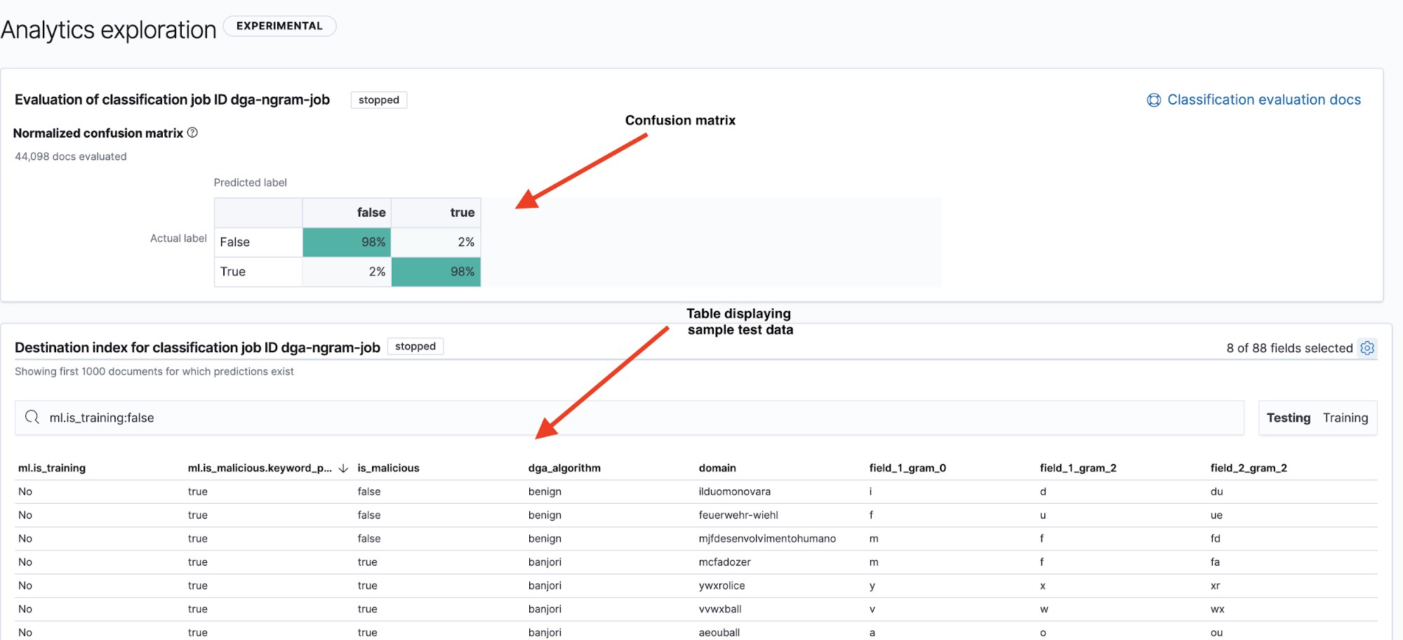
A common way to display a model’s performance is with a visualization known as the confusion matrix. The confusion matrix displays the percentage of data points that were classified as true positives (the malicious domains that the model identified as malicious and that were actually malicious) and true negatives (the benign domains that the model identified as benign), as well as the percentage of documents where the model confused benign domains for malicious (false positives) or vice versa (false negatives).
True to its name, the confusion matrix will quickly show us if a model is frequently confusing instances of one class for another.
In Figure 6, we see that our model has a 98% true positive rate on the testing data. This means that if we were to deploy this model into production to classify incoming DNS data, we would roughly expect to see a 2% false positive rate. Although this seems like a fairly low number, the high volume of DNS traffic means that it would still lead to a fairly high alert rate. In part 2, we will take a look at how anomaly detection can be used to reduce the number of false positive alerts.
Deploying the DGA model into production
Once the model has been trained and evaluated, it is time to think about putting it into production! In the next blog post of this series we will be taking a look at how to create an inference processor and use this along with Ingest Pipelines and packetbeat to detect DGA activity in your network. We will also give options for those users who are not currently using Packetbeat to ingest their network data.
Conclusion
In this blog post, we have taken a brief overview of using Elastic machine learning to build and evaluate a machine learning model for DGA detection. We have examined the process of extracting features from the raw malicious and benign domains and explained a bit about the process of finding suitable features. Finally, we have taken a look at how to train and evaluate a machine learning model using the Elastic Stack.
In the next part of the series, we will take a look at how to use Inference Processors in ingest pipelines to deploy this model to enrich incoming Packetbeat data with predictions of domain maliciousness and how to use anomaly detection jobs to reduce the number of false positive alerts. In the meantime, try our machine learning features out for free to see what sort of insights you can unlock when you see through the noise in your data.