How I used Elastic Maps to plan my cycling trip and find unique roads
.jpg)

 Share on Twitter
Share on Twitter

 Share on LinkedIn
Share on LinkedIn

 Share on Facebook
Share on Facebook

 Share by Email
Share by Email

 Print this page
Print
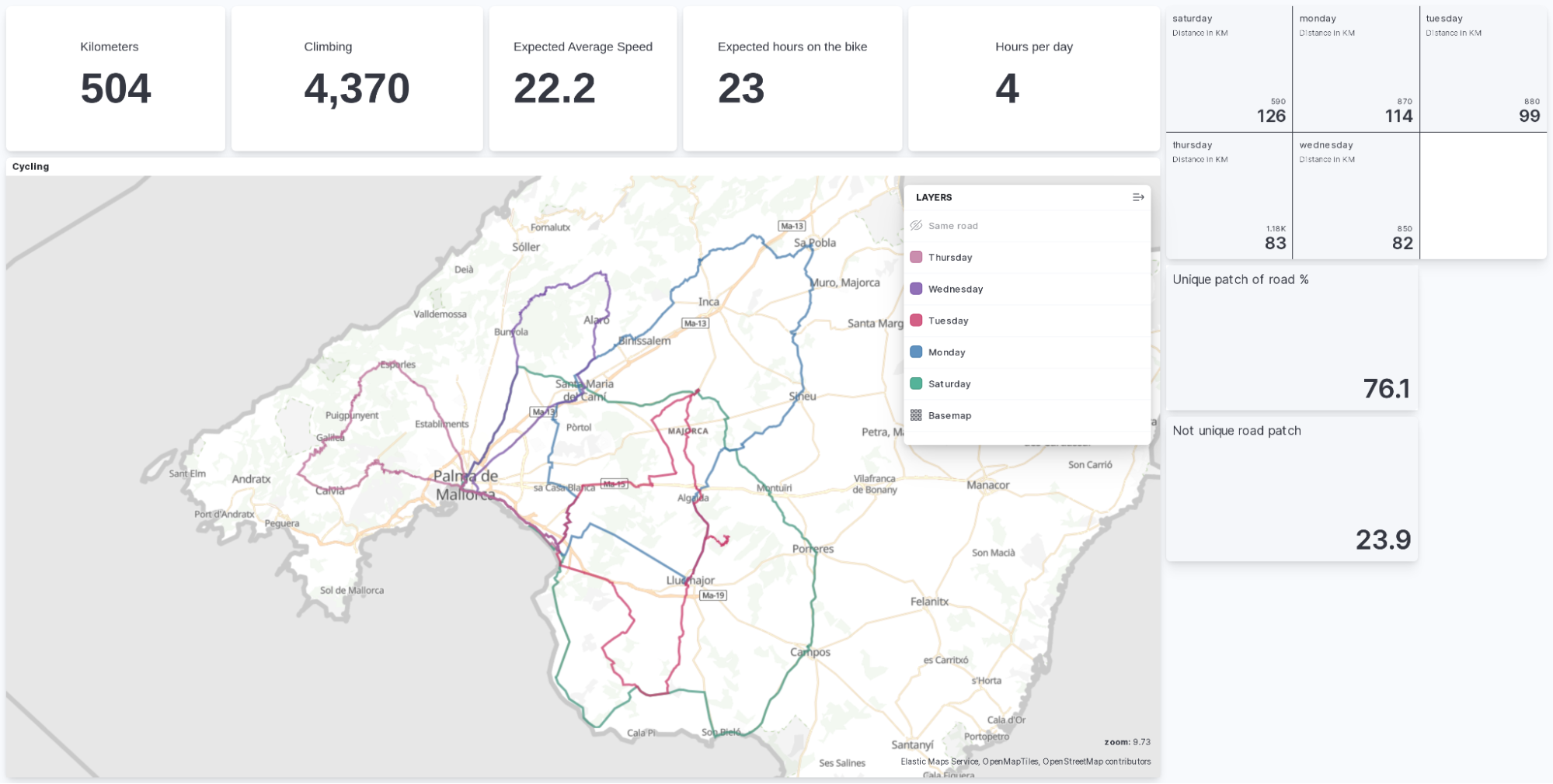
At Elastic, many of our Elasticians love cycling and exploring new and unique patches of road. We also love data analysis and visualization. I started to plan my upcoming cycling trip on Komoot. Planning a one-week trip with six rides is tricky, as you are hovering over the map and trying to find unique routes. Who wants to ride the same road multiple times?
After I was done planning in Komoot, I thought to myself: is there a way to identify if I am riding this road once, twice, or even more often? I also wanted to plot it and look at the data a bit more dynamically.
This is our goal today. Let’s build a dashboard that shows this information.
[Related article: How to use Elastic Maps to make public datasets observable]
Exporting and preparing for import
First, we need to get the GPX file from Komoot. Currently, Elastic cannot read GPX files directly. So, we need to convert them to anything that is supported. I opted for a GeoJSON since I could use the togeojson from Mapbox.
Download the GPX and run the following command after installing togeojson: togeojson 2022-10-10-Thursday.gpx > Thursday.geojson. This should give you a file called Thursday.geojson.
Now we can open that file in any editor, and we will add a few more details. The GPX export does not contain information about the ascent, descent, expected speed, or kilometers covered. I excluded the entire geoJSON and marked multiple data with ...
{
   "type": "FeatureCollection",
   "features": [
       {
           "type": "Feature",
           "properties": {
               "name": "Thursday",
               "time": "2022-10-10T21:21:49.168Z",
               "coordTimes": [
                   "2022-10-10T21:21:49.168Z",
                   "2022-10-10T21:21:52.364Z",
                   "2022-10-10T21:22:06.855Z",
                   "2022-10-10T21:22:16.035Z",
                   "2022-10-10T21:22:24.638Z",
		      …,
                 ]
           },
           "geometry": {
               "type": "LineString",
               "coordinates": [
                   [
                       2.748933,
                       39.515513,
                       8.501845
                   ],
                   [
                       2.748722,
                       39.515419,
                       8.501845
                   ],
                   …
                 ]
           }
       }
   ]
}Within the properties we now want to add additional information. In the end, it should look like this:
   "properties": {
               "name": "Thursday",
               "expected": {
                   "speed": 22,
                   "minutes": 300
               },
               "kilometers": 83,
               "ascent": 1180,
"time": "2022-10-10T21:21:49.168Z",We added expected.speed, expected.minutes, kilometers, and ascent. Important here is that you do not add quotes to the values. Otherwise, Elasticsearch will treat it as a keyword, and you won’t be able to run mathematical calculations like sum, average, etc.
Now that we have laid the groundwork, we can get to the fun part!
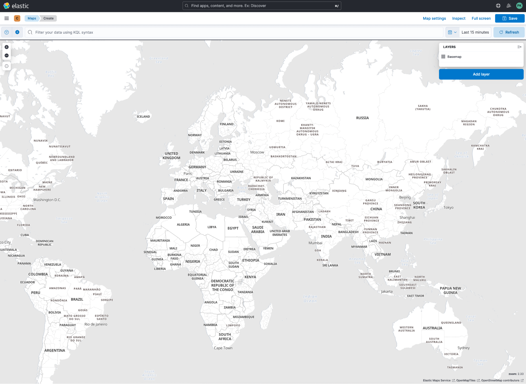
Getting the data onto a map in Kibana
We now go to Kibana and select maps. We are greeted with an empty base map that looks like this:
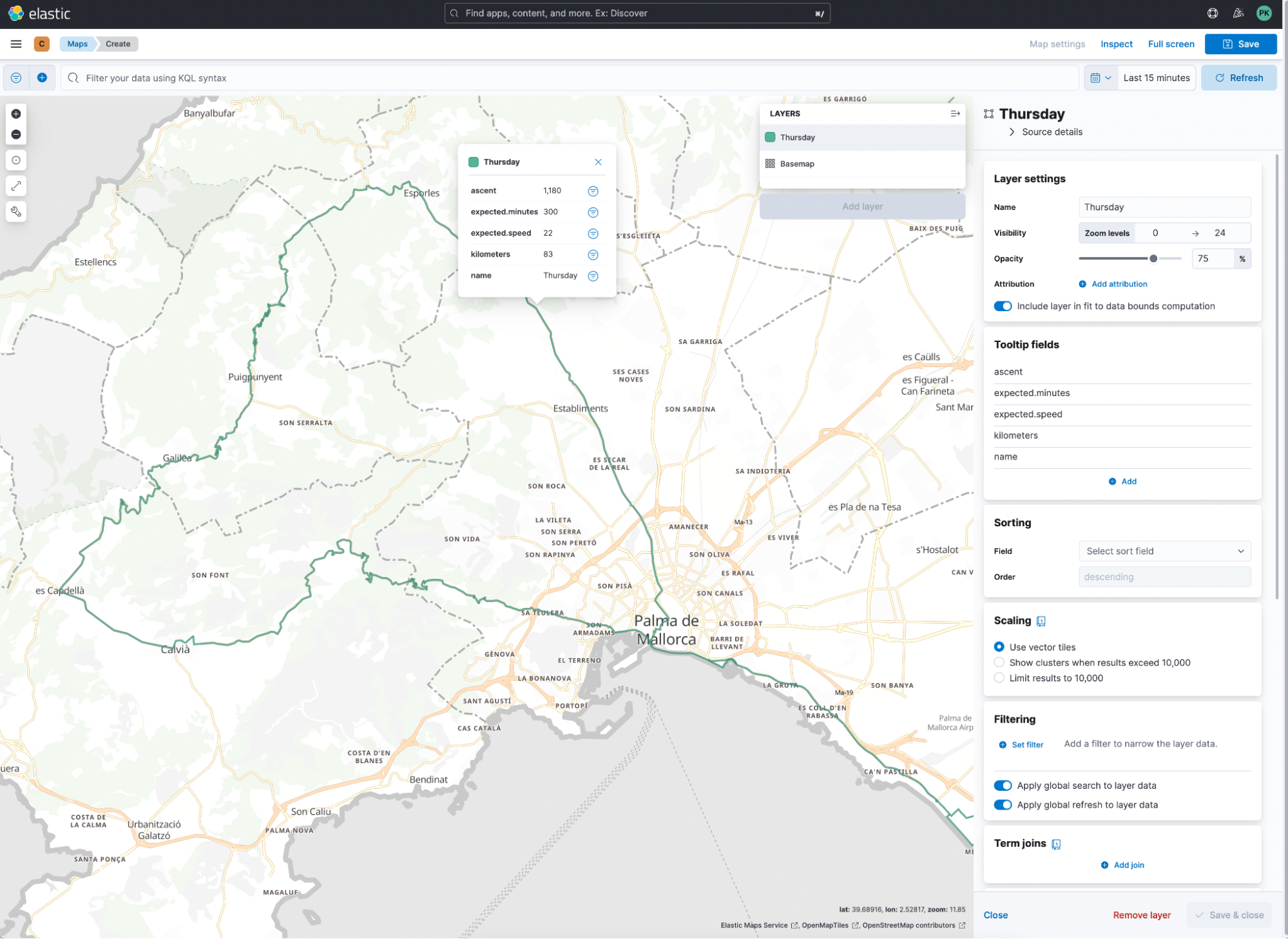
Let’s click on Add Layer and select the file — in my case, it is Thursday. As an index name, I added the prefix c-, but you could add cycling-. This is important since we are uploading every day individually.
We want to look at all the data at once. Therefore, we need a data view that simply does c-*. We want to add a few tooltips like ascent and kilometers in the layer view. Isn’t that already really pretty?
If you enjoy a visual approach more, then take a look at this quick demonstrative video.
The tricky part
When we think back at the start of this blog post and the dashboard we saw, there are simple visualizations, the sum of kilometers, the sum of ascent, and average of expected.speed. All of them can be done quickly in Lens. The tricky part is identifying unique patches of road. I like to spend time riding on roads I’ve never seen before.
Visual confirmation is possible in maps using the clusters option with either clusters or grids as a selection. Every time we see one, we know that there is only one document matching that geo point. Some are riding along the same route multiple times, in the city of Palma and near my hotel.
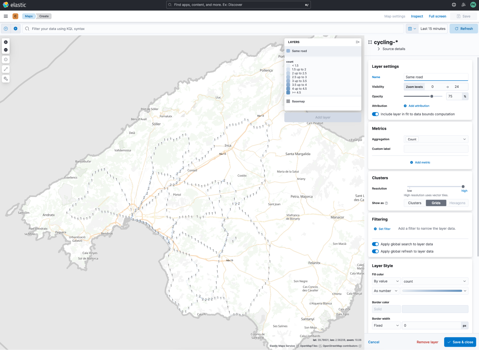
Let’s put this into perspective. According to the map, it is difficult to estimate how much riding is now happening in total, in a percentage view.
This is the part where we need to head over to the Dev Tools in Kibana and write a so-called geotile aggregation. I prepared one — the only thing you might want to change is the precision. This decides how many tiles (squares) Elasticsearch is calculating and then checking if the geo_point is located within that tile.
GET c-*/_search
{
 "size": 0,
 "aggs": {
   "patches": {
     "geotile_grid": {
       "field": "geometry",
       "precision": 20
     }
   }
 }
}The answer contains an aggregation where the key represents the zoom/x/y representation. The doc_count is the interesting part. Since I have uploaded a total of six rides, I would expect the doc_count to be a maximum of 6, meaning that on every ride, I cross this tile.
{
 "took": 53,
 "timed_out": false,
 "_shards": {
   "total": 6,
   "successful": 6,
   "skipped": 0,
   "failed": 0
 },
 "hits": {
   "total": {
     "value": 11,
     "relation": "eq"
   },
   "max_score": null,
   "hits": []
 },
 "aggregations": {
   "patches": {
     "buckets": [
       {
         "key": "20/532297/398803",
         "doc_count": 5
       },
       {
         "key": "20/532296/398804",
         "doc_count": 5
       },
       …
    ]
  }
  }
}We can run a curl request to retrieve that response for the search. You can copy the curl command using the wrench symbol in Dev Tools. Alternatively, you can run the search through Dev Tool and just copy the answer JSON into your text editor and save it.
I copied it from the Dev Tools and saved it as geodata.json. I now need to run JQ, which allows the parsing of JSON files using a command line. I want to convert every key + doc_count pair into its representative line and create an NDJSON file, which I then upload using Kibana. That is the command line you need to run.
cat geodata.json | jq '.aggregations.patches.buckets | .[]' -c > geodata.kibana.ndjson
This creates a geodata.kibana.ndjson file, looking like this:
{"key":"20/532297/398803","doc_count":5}
{"key":"20/532296/398804","doc_count":5}
{"key":"20/532296/398803","doc_count":5}
{"key":"20/532295/398804","doc_count":5}
{"key":"20/532294/398805","doc_count":5}
{"key":"20/532294/398804","doc_count":5}
{"key":"20/532293/398804","doc_count":5}
{"key":"20/532293/398803","doc_count":5}Now head to the file upload function in Kibana, located under Machine Learning > Data Visualizer > File, and upload it. You can name it however you like — I named it cycling-geostats.
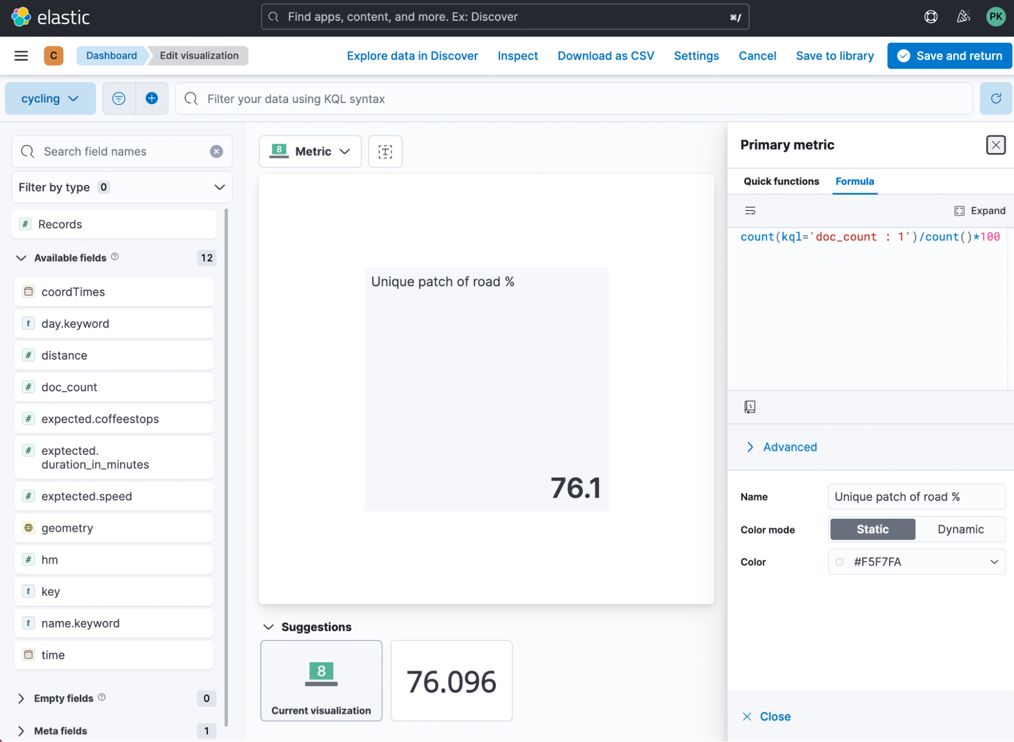
Let’s create a new Lens visualization of the Metric kind and then click on the Primary Metric. We want to create a custom formula, since we need to calculate the following:
- Unique % of road
- Duplicated % of road
For the unique % of road, we can leverage this formula count(kql='doc_count : 1')/count()*100
Let me break it down for you:
- Count all documents where doc_count equals 1. That allows us to get an entire count of all tiles that we cross once.
- Divide by all available tiles.
- Multiply by 100 to get to a percentage view.
This results in the following visualization:
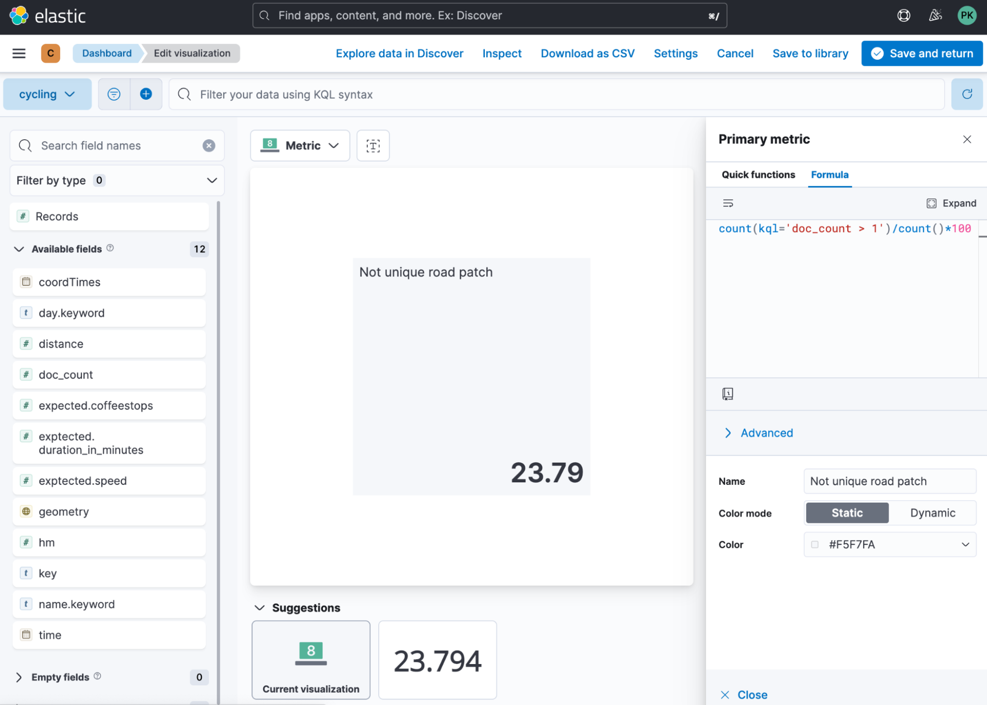
Now we need to do that again but for the duplicated amount of tiles. The formula is nearly identical count(kql='doc_count > 1')/count()*100 . The only difference is that we only look on all tiles where the doc_count is greater than 1. Thus we are crossing it at least two times.
Summary
This blog post covered a few first steps into analyzing and visualizing data using a different example on a small-scale dataset that is easy to digest and understand. This really helped me in planning my cycling trip, and it made a few colleagues intrigued to try it out on a bigger scale by importing all of their Strava rides! One of the next steps would be to add a timestamp to it, and then you can group it by months and seasons. Answering questions like: Which road do I prefer in winter? Is there a lot of overlap between winter and summer?
I hope you all enjoyed it!
Share
- Share on Twitter
Share on Twitter
- Share on LinkedIn
Share on LinkedIn
- Share on Facebook
Share on Facebook
- Share by Email
Share by Email
- Print this page
Print