Feature importance for data frame analytics with Elastic machine learning
With Elasticsearch machine learning one can build regression and classification models for data analysis and inference. Accurate prediction models are often too complex to understand simply by looking at their definition. Using feature importance, introduced in Elastic Stack 7.6, we can now interpret and validate such models.
Motivation
Using data frame analytics (introduced in Elastic Stack 7.4), we can analyze multivariate data using regression and classification. These supervised learning methods train an ensemble of decision trees to predict target fields for new data based on historical observations.
While ensemble models provide good predictive accuracy, this comes at the cost of high complexity. Feature importance gives us a locally-accurate linear model representation of an ensemble model. Thus, it helps us to understand and to interpret the model predictions. There are two questions that feature importance can help us to answer.
First, we can ask whether what the model has learned about the data makes sense? Here, feature importance gives us tools to interpret and to verify the model predictions using domain knowledge. Sometimes, we may see that a feature has little impact on the prediction, and domain knowledge supports this observation. Then we can decide to remove the feature altogether to improve the model.
Second, we can ask ourselves what we can deduce from the learned dependencies between quantities in a data set? In this blog post, we show how one can use feature importance for exploratory data analysis. We’ll use the Elastic machine learning feature importance capability to analyze the World Happiness Report dataset and to discover the reasons for people’s happiness.
If you are interested in more technical details — and not afraid of a little Python — you can follow along using the accompanying Jupyter notebook.
(Data) Framing happiness
Our ML capabilities are most often used in our Security and Observability solutions, but sometimes we just like to have some fun, so we will try to investigate whether "money can buy happiness" using machine learning and feature importance. What are some of the factors that can determine happiness, and which is most important? Will buying a Rolls Royce make you happier? If not, then what will?
Making things more complicated, we know that different nationalities have different mentalities and value different things in life. You may have noticed this if you have lived in different countries or if you were traveling around the world. Yes, everyone has anecdotes, but can this observation be measured empirically? In fact, it can! And the World Happiness Report is a survey that does just that — it ranks 156 countries by how happy their citizens perceive themselves to be.
As a data scientist, I knew I could get to the bottom of my Rolls Royce question.
The World Happiness Report asks citizens of the surveyed countries to say how happy they are on a scale from 0 to 10. Additionally, the survey captures the following information:
- GDP per capita
- Social support
- Healthy life expectancies at birth
- Freedom to make life choices
- Generosity
- Perceptions of corruption
- Positive affection of the respondents
- Negative affection of the respondents
The World Happiness Report for 2019 contains the historical survey data from 2008 through 2018.
Feature importance: Digging a little deeper
Feature importance is similar in concept to influencers in our unsupervised anomaly detection. They both help users to interpret and to more deeply understand (and trust) the results of the analytics. Yet, despite the similarity of these concepts, the implementation details are significantly different.
Within the context of data frame analytics, feature importance can be defined in many different ways. There are general model-independent definitions as well as those specific to decision trees. We use the SHAP (SHapley Additive exPlanations) Algorithm by Lundberg and Lee. This algorithm assigns a SHAP value for every feature in every data point. The sum of these values for a data point gives us the deviation of model prediction from the baseline. The baseline value is the average of predictions for all data points in the training data set.
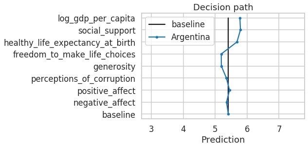
The figure above shows the decision path our model takes when predicting the happiness score of Argentina. The path starts at the baseline of 5.41 and then incrementally adds the feature importance values until it finally results in the predicted happiness score of 5.83. If the decision path goes left, the feature has a negative effect on the model prediction (e.g., generosity). If the decision path goes right, the feature has a positive effect (e.g., healthy_life_expectancy_at_birth).
Every feature importance value affects the decision of the model, increasing or decreasing the prediction. Hence, the features with the largest positive or negative feature importance values — with the largest absolute values — are the most significant for a particular data point.
For classification models, the sum of feature importance values approximates the predicted log-odds. No worries if you don't know what a log-odd is. The takeaway message is that the effects of feature importance for classification can be interpreted in very much the same way as its effects for regression.
Getting started with feature importance
To activate feature importance computation in a data frame analytics job, we need to pass the configuration parameter "num_top_feature_importance_values" in the "analysis" section. The parameter defines the maximum number of feature importance values reported for every data point (see API Reference for details).
Unless you have too many features and may run into the danger of exploding indices, you can set this parameter equal to the number of features in the data set. In our example, we set "num_top_feature_importance_values" to 8.
PUT /_ml/data_frame/analytics/world-happiness-report
{
  "id": "world-happiness-report",
  "description": "",
  "source": {
    "index": [
      "world-happiness-report"
    ],
    "query": {
      "match_all": {}
    }
  },
  "dest": {
    "index": "whr-regression-results",
    "results_field": "ml"
  },
  "analysis": {
    "regression": {
      "dependent_variable": "life_ladder",
      "training_percent": 80,
      "num_top_feature_importance_values": 8
    }
  },
  "analyzed_fields": {
    "includes": [],
    "excludes": [
      "year",
      "country_name"
    ]
  }
}
Then we trigger the analytics job:
POST /_ml/data_frame/analytics/world-happiness-report/_start
Upon job completion, the feature importance values are stored in the destination index in the fields prefixed by “ml.feature_importance.” So, in our example, the feature importance of the field “generosity” is stored in the field “ml.feature_importance.generosity”.
It is likely that, for individual documents, the number of reported feature importance values will be smaller than the number specified in "num_top_feature_importance_values". This happens if a model does not require some features for a prediction: If a feature importance value is zero, it is not reported.
Analyzing the data
Since feature importance is computed for individual data points, we, of course, can aggregate those to average magnitudes over the complete data set and get a quick summary of which features are, in general, more important than others.
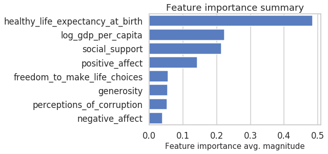
We can immediately see that “healthy_life_expectancy_at_birth” is the most important feature. Also “log_gdp_per_capita” has generally a similar importance to “social_support”.
To dive a little deeper into the details, we can compare the distribution of feature importance values for different features, as shown below. Here, we see a combination of a scatter plot and a violin plot showing the importance values for individual features. Features with higher overall feature importance tend to have a more extensive spread from minimum to maximum.
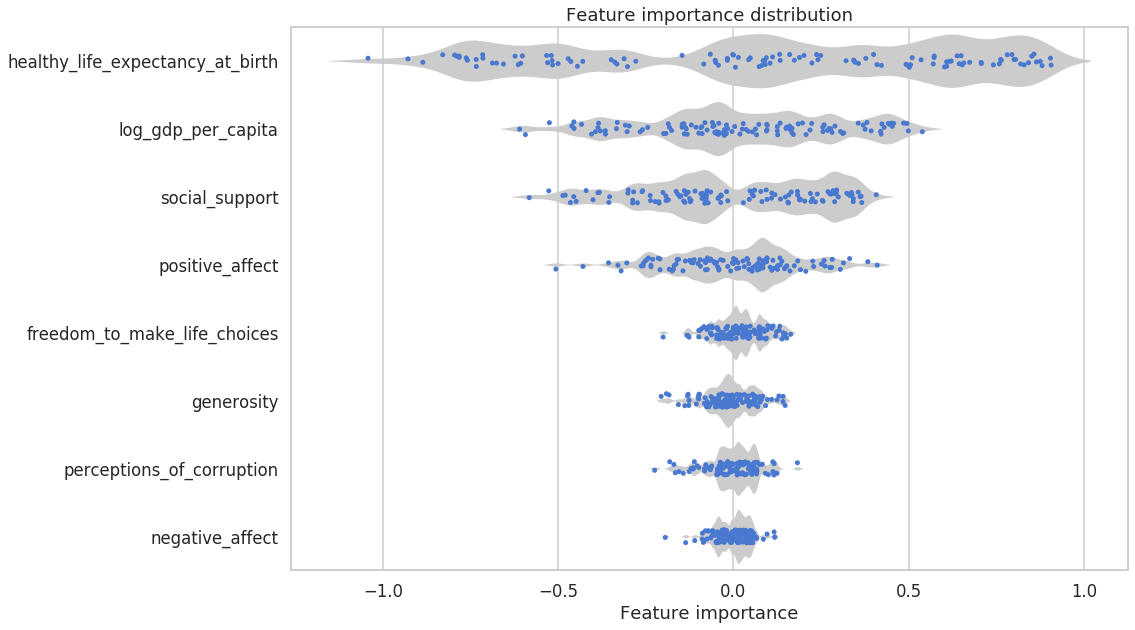
Moreover, the diagram helps us to identify clusters of feature importance values. Indeed, it shows that “healthy_life_expectancy_at_birth” has several groups: On the left side, we have a large concentration of countries where life expectancy has negative feature importance. Those are the countries where low life expectancy reduces the happiness score. On the right side, we have a large concentration of countries where life expectancy has positive feature importance. High life expectancy in those countries increases the happiness score.
For the features “generosity”, “freedom_to_make_life_choices”, “perceptions_of_corruption”, and “negative_affect”, we see a large concentration of countries around 0 mark. For those countries, the features don’t have a significant effect on happiness.
Let’s now “zoom in” on the most distinctive feature “healthy_life_expectancy_at_birth” and look at the dependence plot. This plot shows the distribution of feature importance values as a function of feature values.
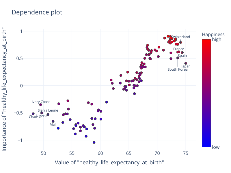
The dependence plot shows a linear relationship: the higher the feature value, the higher its effect on the prediction. We can also see a positive correlation between life expectancy and happiness. In the top right corner we see countries with a higher happiness score (red). Similarly, in the bottom left corner we see countries with a lower happiness score (blue).
However, interestingly and somewhat unexpected is the following observation: the linear dependency does not hold for life expectancy under 57 and over 72. On the right side of the plot, countries like Japan, South Korea, Spain, and France show that although they have a very long life expectancy, this has a comparably low effect on their happiness. Similarly, on the left side of the plot, we see African countries like Chad, Ivory Coast, Sierra Leone, Nigeria, and Mali with the shortest life expectancy but not the strongest negative effect of this feature on their happiness.
Come to think of it, people rarely worry about their life expectancy on a daily basis. This feature serves rather as a proxy for multiple factors such as quality of health care, air pollution, and sanitation. Once these factors are taken care of, life expectancy is affected by factors like genetics and diet, which are less correlated with happiness.
Looking at the same kind of plot for "log_gdp_per_capita", we see again the general correlation between the feature value and the feature importance as well as between the feature value and the happiness score.
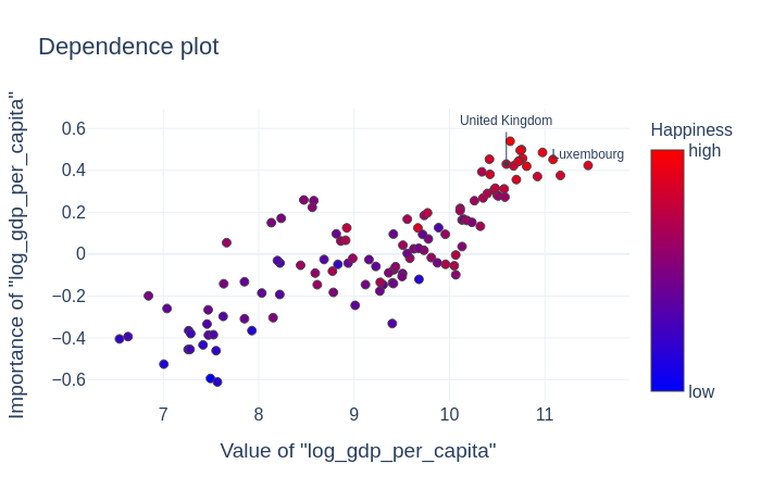
For log GDP over about 10.5 the importance of this feature stagnates and other features become more relevant. For example, although Luxembourg has almost an order of magnitude higher GDP per capita than the United Kingdom, for both these countries, this feature contributes equally to the overall prediction of the happiness score.
Conclusions
Is money important for happiness? It depends. Every country has its unique empirically measurable profile of what makes its citizens happy on a macroscopic level.
Looking at the World Happiness Report, we can conclude that, overall, countries' wealth (as determined by GDP per capita), is only the second most significant factor. It is superseded by the ability to live a long and healthy life. Having a good social network of family and friends and enjoying happy moments in life are the other two important factors (way more important than a Rolls Royce).
We have seen that countries exhibit their individual "happiness profiles." For both most important features — GDP and healthy life expectancy — the importance stagnates at the extreme sides of the spectrum. This means that, for very rich and very poor countries, factors other than wealth become more important.