Interpretability in ML: Identifying anomalies, influencers, and root causes
Machine learning algorithms are becoming more and more integral to many decision making processes in fields ranging from medicine and finance. While augmenting traditional intelligence with insights derived from machine learning algorithms is beneficial, it also introduces a host of questions. Can we be confident that machine learning systems will produce accurate decisions when deployed in critical settings? How easy is it to interpret machine learning models? Can we engineer ways to explain decisions made by these systems?
Not only are such explainability and interpretability features crucial to enshrine trust in machine learning systems, they are also increasingly tied in with data protection regulations. For example, the General Data Protection Regulation (GDPR) introduced in the European Union aims to give data subjects rights to know about automated decisions carried out with their personal data.
At Elastic, we attempt to engineer explanatory facilities into our machine learning products to help users understand which factors could be influencing a particular decision made by a machine learning job. In this post, we’ll attempt to uncover some of the thinking behind anomaly detection influencers, an “explanatory” feature that we developed to help users understand the anomalies picked out by our anomaly detection algorithm.
Engineering explanations in anomaly detection
Users of our anomaly detection product will be familiar with influencers — values that affect or influence a given anomaly. Let’s take a look at how we compute these values.
Consider a fictional corporate network where the number of bytes sent by a machine’s communication applications (Skype, Messenger, Outlook) are tracked to make sure that unusual or malicious data exfiltration can be identified. We want to run anomaly detection on the number of bytes to make sure we are alerted if the number exceeds the mean (potential data exfiltration) or falls below the mean (potential malfunction in some part of the network). The time series profile of our dataset could look like something from Figure 1.
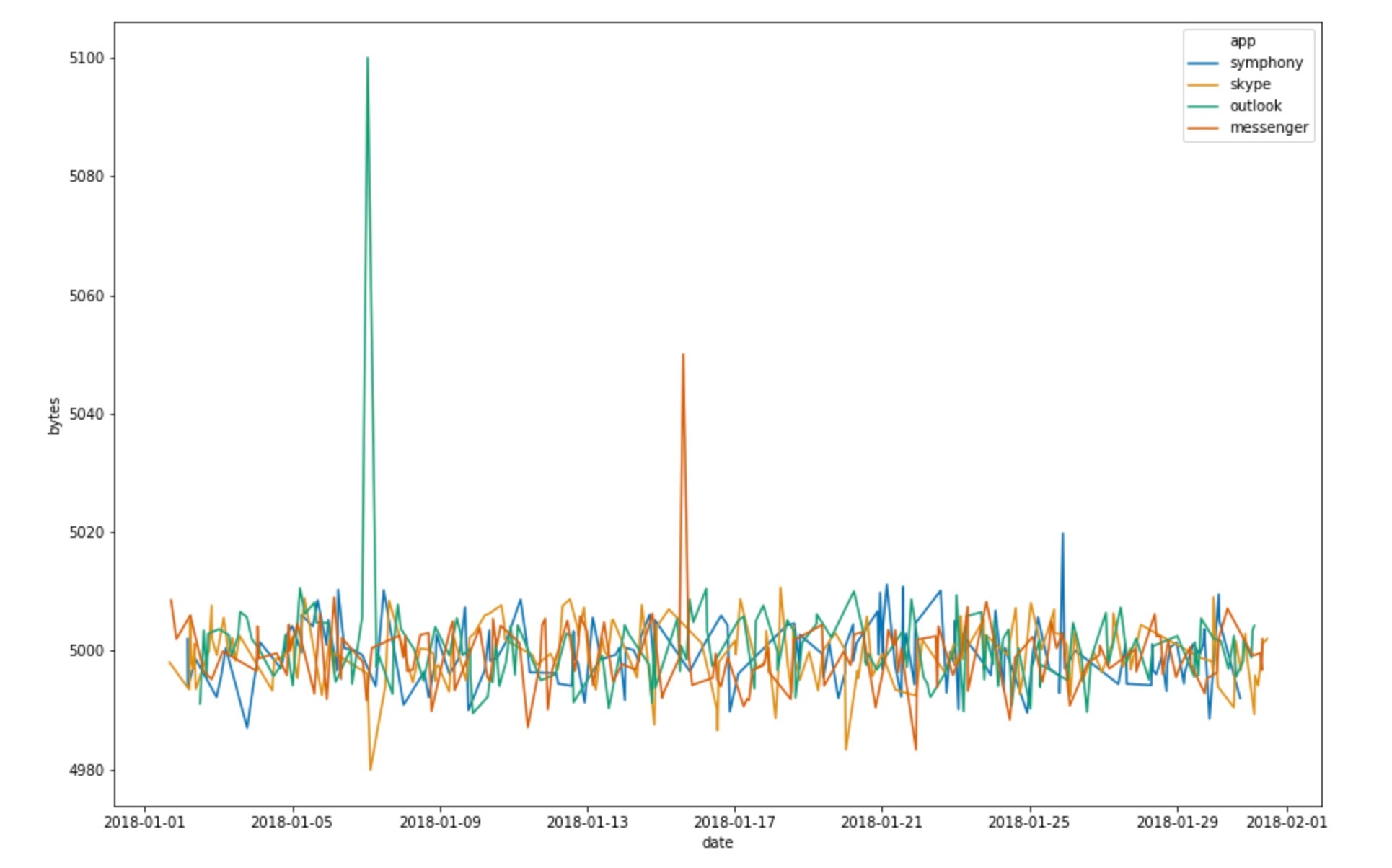
Figure 1: Time series profile of bytes sent by different applications in a corporate network
We have various applications sending bytes over the corporate network. When we configure our bucket span, let’s say 12 hours, and apply our detector function, let’s say mean, we transform the dataset to look something like the time series in Figure 2. This is a simplified case to help in illustrating the concept of influencers and simplifies many of the complexities needed in a production machine learning job. For example, in a case like this in a production system, one might want to model the time series profile of each application separately.
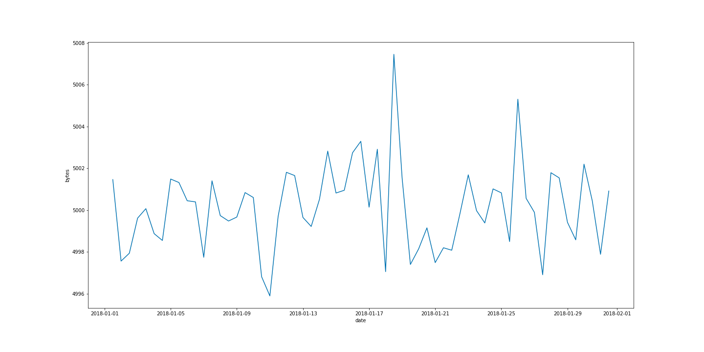
Figure 2: Time series profile of mean bytes sent on a corporate network grouped into 12 hour buckets.
Each individual bucket value becomes a datapoint that we use to create various distributions to model the behavior of the network. As we can see from Figure 3, the distribution profile of our model mean bytes evolves the more data the anomaly detection system sees.
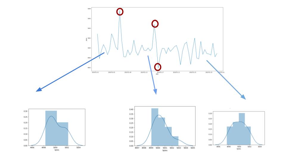
Figure 3: The distribution that models the individual bucket values evolves as it sees more time series data.
When we encounter a bucket value that has a very low probability of occurring according to our model of the data at that point in time, we mark the bucket as anomalous.
But what can we say caused the anomaly at that point in time? Inferring causation from correlation is a notoriously thorny problem. For example, consider we were tracking the sales of sunglasses and ice cream and if we lived on a planet without summers, just observing a plot of sales of sunglasses versus sales of ice cream might lead us to infer that an increase in the amount of ice cream causes people to desire more sunglasses, when in fact the increase in the sales of both is caused by the warm summer temperatures. Therefore, a key part of inferring or even suggesting causation is domain knowledge. Hence when you configure an anomaly detection job, we ask the user who likely has the most domain knowledge to specify which entities in the dataset would be the likely causes of any irregularities.
A tale of two thought experiments
To determine which entities caused a given bucket to exhibit anomalous behaviors, we turn to two strategies, which both involve asking “what if” questions. Let’s first take a look at detector functions such as mean, count, and sum that are additive in nature; that is, they add up all of the individual datapoints in a bucket to compute the final number, which will be used to perform anomaly detection.
For these kinds of functions, to determine which of the influencer fields could be a potential explanation for an anomaly in a given bucket, we use so called counterfactual causation reasoning. Imagine for a second that the bucket marked in Figure 4 has scored a very low probability for mean bytes. The anomaly detection algorithm examines each of the datapoints present in the bucket and then groups them according to the value of the influencer. In the case of applications sending bytes over a corporate network, a natural candidate for an influencer value is the name of the application. Thus, we take the anomalous bucket and group the datapoints according to which app (Skype, Messenger, Outlook) generated them.
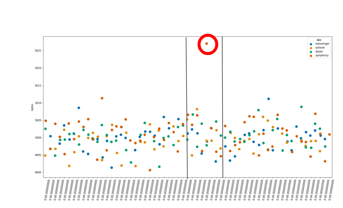
Figure 4: The anomaly detection algorithm keeps track of the influencer values in each bucket and can use those to assign blame for anomalous buckets.
Then, for each of the possible apps, we remove the datapoints corresponding to the app and check to see if the bucket’s value is still anomalous with the datapoints removed. If the value is no longer anomalous after these datapoints have been removed, we can conclude that this value for the app has something to do with the bucket’s value being anomalous. If, on the other hand, the bucket is still anomalous even with the values removed, it appears that this particular app does not explain the anomaly.
Unfortunately, reasoning about what happens if some of the data were removed can only provide explanations when the anomalous value is higher than the expected value. If the value is lower, we cannot use this type of reasoning to discover which values should be in the bucket, but are missing, and thus causing the anomaly.
We also cannot use this type of reasoning for detector functions like min or max. Consider for a moment that we're interested in tracking anomalies in the number of max bytes sent in our example corporate network, and the typical values for the max bytes is 5,000 bytes over some period of time. Now suppose all of a sudden, the value in the bucket jumps to 10,000 bytes. When we examine the apps active in the bucket, we find two possible explanations. Both Skype and Messenger are sending 10,000 bytes in this bucket.
Now, applying the logic we developed for counterfactual causation, to this situation, we get the following. Suppose we remove all datapoints generated by Skype. The max value of the bucket would still be 10,000 bytes, because the datapoints generated by Messenger are still in the bucket. According to the counterfactual causation reasoning, Skype is thus not an influencer for the anomaly because the anomalousness of the bucket did not change when we removed datapoints generated by Skype. A symmetrical argument can also be applied to the datapoints generated by Messenger. The result of this reasoning would indicate that neither Skype nor Messenger are responsible for the anomaly, which conflicts with our intuition.
Therefore, for functions like max and min, we deploy a mode of reasoning we call regularization. Unlike in counterfactual causation, in regularization, for each possible value of the influencer, we restrict the anomalous bucket to contain only datapoints generated by the given value. In the case above, we would restrict the bucket to only contain datapoints generated by Skype. If the bucket value is still anomalous after we restrict the set of datapoints to only contain datapoints from the given influencer candidate, then we can say that this influencer explains the anomaly. Please note, that an anomaly can have more than one influencer.
One challenge with the strategies described above is that they are less effective if data is pre-aggregated before it is analyzed by the anomaly detection system. For example, suppose that prior to ingestion we pre-computed the mean of the bytes sent by each application on the corporate network and ingested the data without the information about the originating application (Skype, Messenger, and so on). This would make it impossible to uncover influencers for an anomaly.
Conclusion
When a machine learning system is used to augment existing decision-making processes, it is important to understand what factors influence it to come to a particular decision. In our anomaly detection product, this involves uncovering influencers — fields in the data that affect the anomalousness of the time series we are analyzing online and at scale. If you are interested in learning more about how we score influencers, please be sure to check out this blog post.