Machine Learning Anomaly Scoring and Elasticsearch - How it Works
Editor's Note (August 3, 2021): This post uses deprecated features. Please reference the map custom regions with reverse geocoding documentation for current instructions.
Elastic machine learning anomaly scoring has been updated in Elastic Stack 6.5. Read our anomaly scoring update blog to understand how these changes relate to the normalization of partitions and multi-bucket anomalies.
We often get questions about Elastic's Machine Learning “anomaly score” and how the various scores presented in the dashboards relate to the “unusualness” of individual occurrences within the data set. It can be very helpful to understand how the anomaly score is manifested, what it depends on, and how one would use the score as an indicator for proactive alerting. This blog, while perhaps not the full definitive guide, will aim to explain as much practical information as possible about the way that Machine Learning (ML) does the scoring.
The first thing to recognize is that there are three separate ways to think about (and ultimately score) “unusualness” - the scoring for an individual anomaly (a “record”), the scoring for an entity such as a user or IP address (an “influencer”), and the scoring for a window of time (a “bucket”). We will also see how these different scores relate to each other in a kind of hierarchy.
Record Scoring
The first type of scoring, at the lowest level of the hierarchy, is the absolute unusualness of a specific instance of something occurring. For example:
- The rate of failed logins for user=admin was observed to be 300 fails in the last minute
- The value of the response time for a specific middleware call just jumped to be 300% larger than usual
- The number of orders being processed this afternoon is much lower than what it is for a typical Thursday afternoon
- The amount of data being transferred to a remote IP address is much more than the amount being transferred to other remote IPs
Each of the above occurrences has a calculated probability, a value that is calculated very precisely (to a value as small as 1e-308) - based upon the observed past behavior which has constructed a baseline probability model for that item. However, this raw probability value, while certainly useful, can lack some contextual information like:
- How does the current anomalous behavior compare to past anomalies? Is it more or less unusual than past anomalies?
- How does this item’s anomalousness compare to other potentially anomalous items (other users, other IP addresses, etc.)?
Therefore, to make it easier for the user to understand and prioritize, ML normalizes the probability such that it ranks an item’s anomalousness on a scale from 0-100. This value is presented as the “anomaly score” in the UI.
To provide further context, the UI attaches one of four “severity” labels to anomalies according to their score - “critical” for scores between 75 and 100, “major” for scores of 50 to 75, “minor” for 25 to 50, and “warning” for 0 to 25, with each severity denoted by a different color.
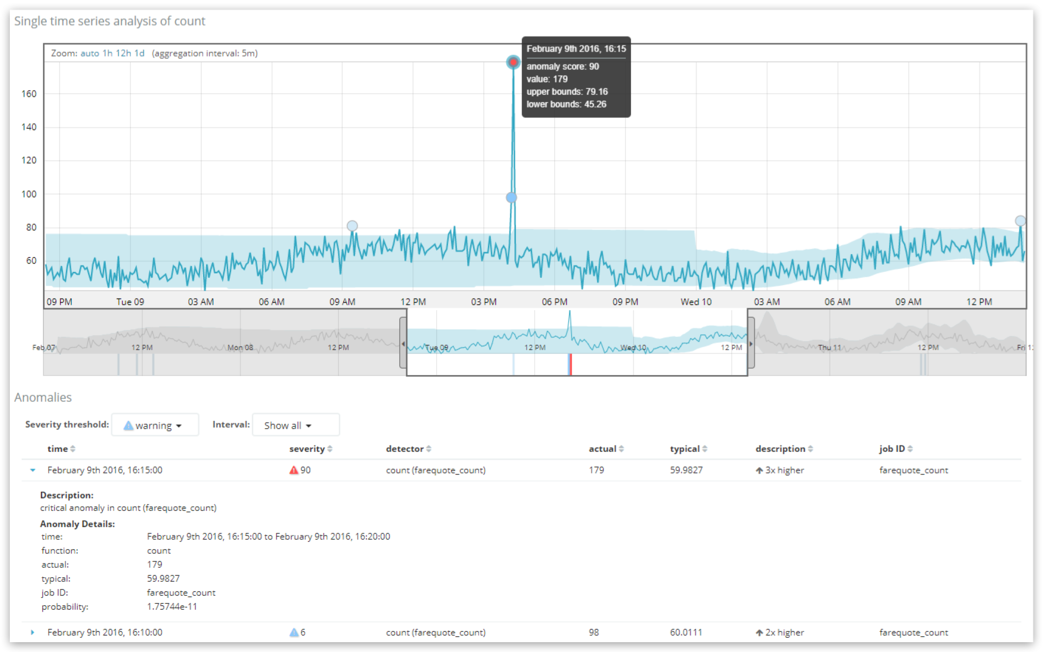
Here we see two anomaly records displayed in the Single Metric Viewer, with the most anomalous record being a “critical” anomaly with a score of 90. The “Severity threshold” control above the table can be used to filter the table for higher severity anomalies, whilst the “Interval” control can be used to group the records to show the highest scoring record per hour or day.
If we were to query for record results in ML’s API to ask for information about anomalies in a particular 5 minute time bucket (where farequote_count was the name of the job):
GET /_xpack/ml/anomaly_detectors/farequote_count/results/records?human
{
  "sort": "record_score",
  "desc": true,
  "start": "2016-02-09T16:15:00.000Z",
  "end" :"2016-02-09T16:20:00.000Z"
}
We would see the following output:
{
  "count": 1,
  "records": [
    {
      "job_id": "farequote_count",
      "result_type": "record",
      "probability": 1.75744e-11,
      "record_score": 90.6954,
      "initial_record_score": 85.0643,
      "bucket_span": 300,
      "detector_index": 0,
      "is_interim": false,
      "timestamp_string": "2016-02-09T16:15:00.000Z",
      "timestamp": 1455034500000,
      "function": "count",
      "function_description": "count",
      "typical": [
        59.9827
      ],
      "actual": [
        179
      ]
    }
  ]
}
Here we can see that during this 5-minute interval (the bucket_span of the job) the record_score is 90.6954 (out of 100) and the raw probability is 1.75744e-11. What this is saying is that it is very unlikely that the volume of data in this particular 5 minute interval should have an actual rate of 179 documents because “typically” it is much lower, closer to 60.
Notice how the values here map to what’s shown to the user in the UI. The probability value of 1.75744e-11 is a very small number, meaning it is very unlikely to have happened, but the scale of the number is non-intuitive. This is why projecting it onto a scale from 0 to 100 is more useful. The process by which this normalization happens is proprietary, but is roughly based on a quantile analysis in which probability values historically seen for anomalies in this job are ranked against each other. Simply put, the lowest probabilities historically for the job get the highest anomaly scores.
A common misconception is that the anomaly score is directly related to the deviation articulated in the “description” column of the UI (here “3x higher”). The anomaly score is purely driven by the probability calculation. The “description” and even the typical value are simplified bits of contextual information in order to make the anomaly easier to understand.
Influencer Scoring
Now that we’ve discussed the concept of an individual record’s score, the second way to consider unusualness is to rank or score entities that may have contributed to an anomaly. In ML, we refer to these contributing entities as “influencers”. In the above example, the analysis was too simple to have influencers - since it was just a single time series. In more complex analyses, there are possibly ancillary fields that have impact on the existence of an anomaly.
For example, in an analysis of a population of users’ internet activity, in which the ML job looks at unusual bytes sent and unusual domains visited, you could specify “user” as a possible influencer since that is the entity that is “causing” the anomaly to exist (something has to be sending those bytes to a destination domain). An influencer score will be given to each user, dependent on how anomalous each was considered in one or both of these areas (bytes sent and domains visited) during each time interval.
The higher the influencer score, the more that entity will have contributed to, or is to blame for, the anomalies. This provide a powerful view into the ML results, particularly for jobs with more than one detector.
Note that for all ML jobs, a built-in influencer called bucket_time is always created in addition to any influencers added during creation of the job. This uses an aggregation of all the records in the bucket.
In order to demonstrate an example of influencers, an ML job is set up with two detectors on a data set of API response time calls for an airline airfare quoting engine:
countof API calls, split/partitioned onairlinemean(responsetime)of the API calls, split/partitioned onairline
with airline specified as an influencer.
Taking a look at the results in the “Anomaly Explorer”:
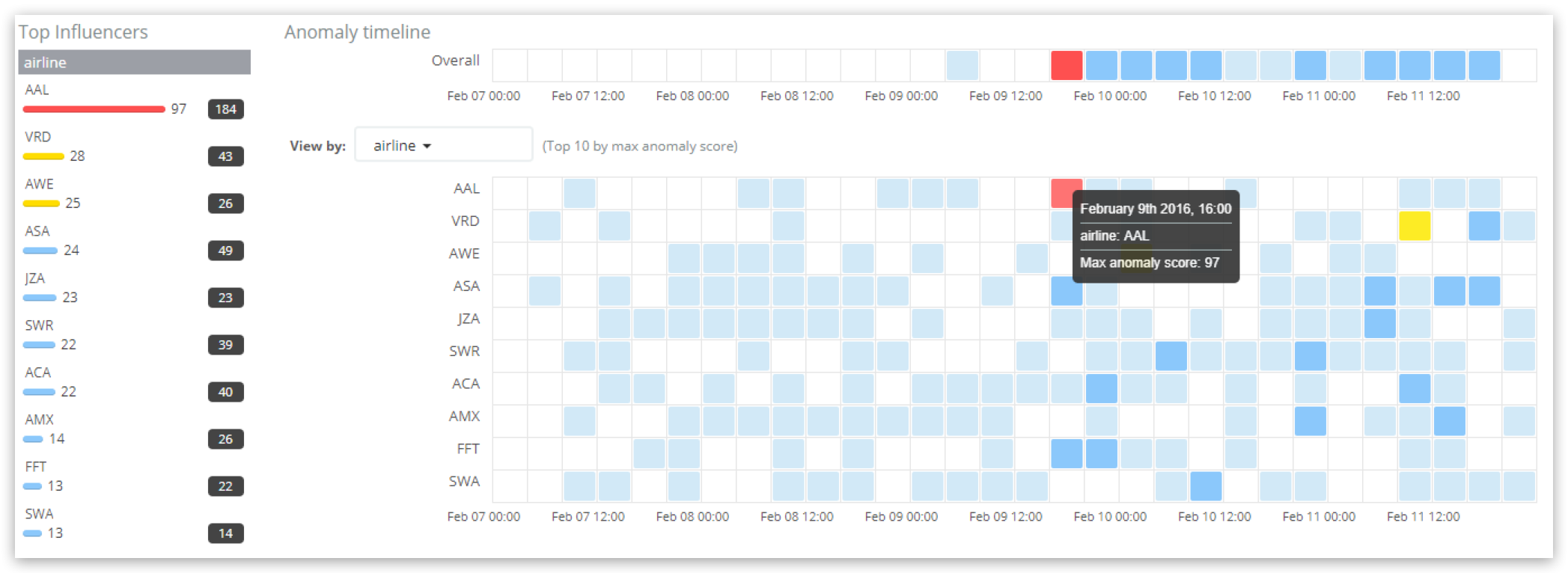
The top scoring influencers over the time span selected in the dashboard are listed in the “Top influencers” section on the left. For each influencer, the maximum influencer score (in any bucket) is displayed, together with the total influencer score over the dashboard time range (summed across all buckets). Here, airline “AAL” has the highest influencer score of 97, with a total influencer score sum of 184 over the whole time range. The main timeline is viewing the results by influencer and the highest scoring influencer airline is highlighted, again showing the score of 97. Note the scores shown in the “Anomalies” charts and table for airline AAL will be different to its influencer score, as they display the “record scores” of the individual anomalies.
When querying the API at the influencer level:
GET _xpack/ml/anomaly_detectors/farequote_count_and_responsetime_by_airline/results/influencers?human
{
  "start": "2016-02-09T16:15:00.000Z",
  "end" :"2016-02-09T16:20:00.000Z"
}
the following information is returned:
{
  "count": 2,
  "influencers": [
    {
      "job_id": "farequote_count_and_responsetime_by_airline",
      "result_type": "influencer",
      "influencer_field_name": "airline",
      "influencer_field_value": "AAL",
      "airline": "AAL",
      "influencer_score": 97.1547,
      "initial_influencer_score": 98.5096,
      "probability": 6.56622e-40,
      "bucket_span": 300,
      "is_interim": false,
      "timestamp_string": "2016-02-09T16:15:00.000Z",
      "timestamp": 1455034500000
    },
    {
      "job_id": "farequote_count_and_responsetime_by_airline",
      "result_type": "influencer",
      "influencer_field_name": "airline",
      "influencer_field_value": "AWE",
      "airline": "AWE",
      "influencer_score": 0,
      "initial_influencer_score": 0,
      "probability": 0.0499957,
      "bucket_span": 300,
      "is_interim": false,
      "timestamp_string": "2016-02-09T16:15:00.000Z",
      "timestamp": 1455034500000
    }
  ]
}
The output contains a result for the influencing airline AAL, with the influencer_score of 97.1547 mirroring the value displayed in the Anomaly Explorer UI (rounded to 97). The probability value of 6.56622e-40 is again the basis of the influencer_score (before it gets normalized) - it takes into account the the probabilities of the individual anomalies that particular airline influences, and the degree to which it influences them.
Note that the output also contains an initial_influencer_score of 98.5096, which was the score when the result was processed, before subsequent normalizations adjusted it slightly to 97.1547. This occurs because the ML job processes data in chronological order and never goes back to re-read older raw data to analyze/review it again. Also note that a second influencer, airline AWE, was also identified, but its influencer score is so low (rounded to 0) that it should be ignored in a practical sense.
Because the influencer_score is an aggregated view across multiple detectors, you will notice that the API does not return the actual or typical values for the count or the mean of response times. If you need to access this detailed information, then it is still available for the same time period as a record result, as shown before.
Bucket Scoring
The final way to score unusualness (at the top of the hierarchy) is to focus on time, in particular, the bucket_span of the ML job. Unusual things happen at specific times and it is possible that one or more (or many) items can be unusual together at the same time (within the same bucket).
Therefore, the anomalousness of a time bucket is dependent on several things:
- The magnitude of the individual anomalies (records) occurring within that bucket
- The number of individual anomalies (records) occurring within that bucket. This could be many if the job has “splitting” using byfields and/or partitionfields - or if there exist multiple detectors in the job.
Note that the calculation behind the bucket score is more complex than just a simple average of all the individual anomaly record scores, but will have a contribution from the influencer scores in each bucket.
Referencing back to our ML job from the last example, with the two detectors:
count, split/partitioned onairlinemean(responsetime), split/partitioned onairline
When looking at the “Anomaly Explorer”
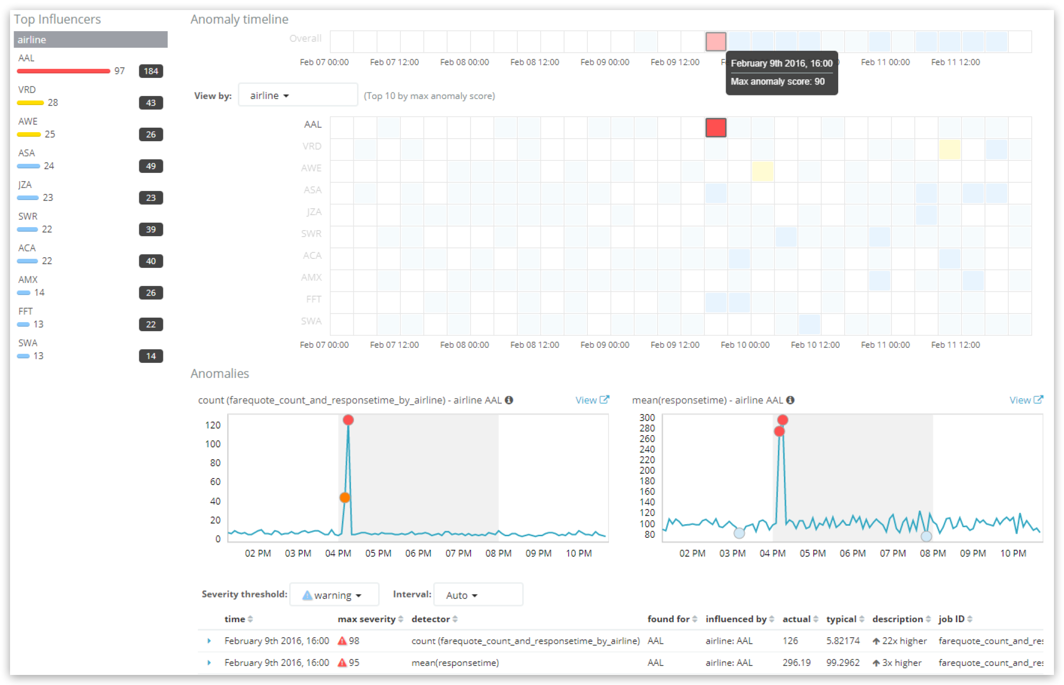
Notice that the “overall” lane in the “Anomaly timeline” at the top of the view displays the score for the bucket. Be careful, however. If the time range selected in the UI is broad, but the ML job’s bucket_span is relatively short, then one “tile” on the UI may actually be multiple buckets aggregated together.
The selected tile shown above has a score of 90, and that there are two critical record anomalies in this bucket, one for each detector with record scores of 98 and 95.
When querying the API at the bucket level:
GET _xpack/ml/anomaly_detectors/farequote_count_and_responsetime_by_airline/results/buckets?human
{
  "start": "2016-02-09T16:15:00.000Z",
  "end" :"2016-02-09T16:20:00.000Z"
}
the following information is present:
{
  "count": 1,
  "buckets": [
    {
      "job_id": "farequote_count_and_responsetime_by_airline",
      "timestamp_string": "2016-02-09T16:15:00.000Z",
      "timestamp": 1455034500000,
      "anomaly_score": 90.7,
      "bucket_span": 300,
      "initial_anomaly_score": 85.08,
      "event_count": 179,
      "is_interim": false,
      "bucket_influencers": [
        {
          "job_id": "farequote_count_and_responsetime_by_airline",
          "result_type": "bucket_influencer",
          "influencer_field_name": "airline",
          "initial_anomaly_score": 85.08,
          "anomaly_score": 90.7,
          "raw_anomaly_score": 37.3875,
          "probability": 6.92338e-39,
          "timestamp_string": "2016-02-09T16:15:00.000Z",
          "timestamp": 1455034500000,
          "bucket_span": 300,
          "is_interim": false
        },
        {
          "job_id": "farequote_count_and_responsetime_by_airline",
          "result_type": "bucket_influencer",
          "influencer_field_name": "bucket_time",
          "initial_anomaly_score": 85.08,
          "anomaly_score": 90.7,
          "raw_anomaly_score": 37.3875,
          "probability": 6.92338e-39,
          "timestamp_string": "2016-02-09T16:15:00.000Z",
          "timestamp": 1455034500000,
          "bucket_span": 300,
          "is_interim": false
        }
      ],
      "processing_time_ms": 17,
      "result_type": "bucket"
    }
  ]
}
Notice, especially, in the output the following:
anomaly_score- the overall aggregated, normalized score (here 90.7)initial_anomaly_score- theanomaly_scoreat the time the bucket was processed (again, in case later normalizations have changed theanomaly_scorefrom its original value). Theinitial_anomaly_scoreis not shown anywhere in the UI.bucket_influencers- an array of influencer types present in this bucket. As suspected, given our discussion of influencers above, this array contains entries for bothinfluencer_field_name:airlineandinfluencer_field_name:bucket_time(which is always added as a built-in influencer). The details of what specific influencers values (i.e. which airline) is available when one queries the API specifically for the influencer or record values, as shown earlier.
Using Anomaly Scores for Alerting
So, if there are three fundamental scores (one for individual records, one for influencers, and one for the time bucket), then which would be useful for alerting? The answer is that it depends on what you are trying to accomplish and the granularity, and thus rate, of alerts that you wish to receive.
If on one hand, you are attempting to detect and alert upon significant deviations in the overall data set as a function of time, then the bucket-based anomaly score is likely most useful to you. If you want to be alerted on the most unusual entities over time, then you should consider using influencer_score. Or, if you are attempting to detect and alert upon the most unusual anomaly within a window of time, you might be better served by using the individual record_score as the basis for your reporting or alerting.
To avoid alert overload, we recommend using the bucket-based anomaly score because it is rate limited, meaning that you’ll never get more than 1 alert per bucket_span. On the other hand if you focus on alerting using the record_score, the number of anomalous records per unit time is arbitrary - with the possibility that there could be many. Keep this in mind if you are alerting using the individual record scores.
Additional reading: