Elasticsearch caching deep dive: Boosting query speed one cache at a time
Cache is king for speedy data retrieval. So if you’re interested in how Elasticsearch leverages various caches to ensure you are retrieving data as fast as possible, buckle up for the next 15 minutes and read through this post. This blog will shed some light on various caching features of Elasticsearch that help you to retrieve data faster after initial data accesses. Elasticsearch is a heavy user of various caches, but in this post we'll only be focusing on:
- Page cache (sometimes called the filesystem cache)
- Shard-level request cache
- Query cache
You will learn what each of these caches is doing, how it works, and which cache is best for which use case. We'll also explore how sometimes you can control the caching and sometimes you have to trust another component to do a good job of caching.
We'll also take a look how page caches deal with expiration of data. One thing you never want to encounter is a cache that returns stale data. A cache has to be bound to the lifecycle of your data and we will take a look how this works for each of them.
And if you're wondering if this post is applicable to you, it doesn’t matter whether you are running Elasticsearch yourself or using Elastic Cloud — you will utilize these caches out of the box. Ok, let's dive in.
Page cache
The first cache exists on the operating system level. While this section is mainly about the Linux implementation, other operating systems have a similar feature.
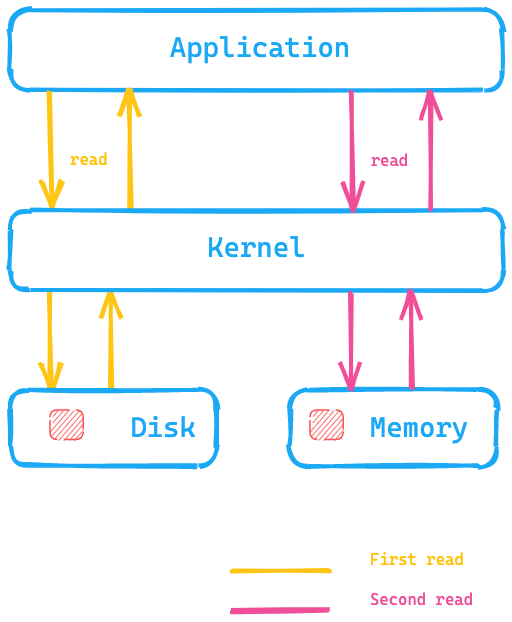
The basic idea of the page cache is to put data into the available memory after reading it from disk, so that the next read is returned from the memory and getting the data does not require a disk seek. All of this is completely transparent to the application, which is issuing the same system calls, but the operating system has the ability to use the page cache instead of reading from disk.
Let's take a look at this diagram, where the application is executing a system call to read data from disk, and the kernel/operating system would go to disk for the first read and put the data into the page cache into memory. A second read then could be redirected by the kernel to the page cache within the operating system memory and thus would be much faster.
What does this mean for Elasticsearch? Instead of accessing data on-disk, the page cache can be much faster to access data. This is one of the reasons why the recommendation for Elasticsearch memory is generally not more than half of your total available memory — so the other half can be used for the page cache. This also means that no memory is wasted; rather, it’s reused for the page cache.
How does data expire out of the cache? If the data itself is changed, the page cache marks that data as dirty and it will be released from the page cache. As segments with Elasticsearch and Lucene are only written once, this mechanism fits very well the way data is stored. Segments are read-only after the initial write, so a change of data might be a merge or the addition of new data. In that case, a new disk access is needed. The other possibility is the memory getting filled up. In that case, the cache will behave similarly to an LRU as stated by the kernel documentation.
Testing the page cache
If you want to check out the functionality of the page cache, we can use hyperfine to do so. hyperfine is a CLI benchmarking tool. Let's create a file with a size of 10MB via dd
dd if=/dev/urandom of=test1 bs=1M count=10
If you want to run the above using macOS, you may want to use gdd instead
and ensure that coreutils is installed via brew.
# for Linux
hyperfine --warmup 5 'cat test1 > /dev/null' \
  --prepare 'sudo sync; sudo echo 3 > /proc/sys/vm/drop_caches'
# for osx
hyperfine --warmup 5 'cat test1 > /dev/null' --prepare 'sudo purge'
Benchmark #1: cat test1 > /dev/null
  Time (mean ± σ):      38.1 ms ±   6.4 ms    [User: 1.4 ms, System: 17.5 ms]
  Range (min … max):    30.4 ms …  50.5 ms    10 runs
hyperfine --warmup 5 'cat test1 > /dev/null'
Benchmark #1: cat test1 > /dev/null
  Time (mean ± σ):       3.8 ms ±   0.6 ms    [User: 0.7 ms, System: 2.8 ms]
  Range (min … max):     2.9 ms …   7.0 ms    418 runs
So, under my local macOS instance running the same cat command without clearing the page cache is about 10x faster, as disk access can be skipped. You definitely want this kind of access pattern for your Elasticsearch data!
Diving deeper
The class responsible for reading a Lucene index is the HybridDirectory class. Based on the extension of files within a Lucene index there is a decision whether to use memory mapping or regular file access using Java NIO.
Also note that some applications are more aware of their own access patterns and come with their own very specific and optimized caches, and the page cache would probably work against that. If needed, any application can bypass the page cache using O_DIRECT when opening a file. We will get back to this at the very end of this post.
If you want to check for the cache hit ratio you can use cachestat which is part of perf-tools.
One last thing about Elasticsearch here. You can configure Elasticsearch to preload data into the page cache via the index settings. Consider this an expert setting and be careful with this setting in order to ensure that the page cache does not get thrashed consistently.
Summary
The page cache helps to execute arbitrary searches faster by loading complete index data structures in the main memory of your operating system. There is no more granularity and it is solely based on the access pattern of your data. The operating system takes care of eviction.
Let's go to the next level of caches.
Shard-level request cache
This cache helps a lot in speeding Kibana up by caching search responses consisting only of aggregations. Let's overlay the response of an aggregation with the data fetched from several indices to visualize the problem that is solved with this cache.
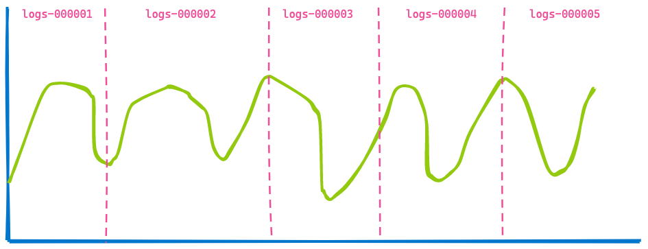
A Kibana dashboard in your office usually displays data from several indices, and you simply specify a timespan like the last 7 days. You do not care how many indices or shards are queried. So, if you are using data streams for your time-based indices you may end up with a visualization like this covering five indices.
Now, let's jump 3 hours in the future, displaying the same dashboard:
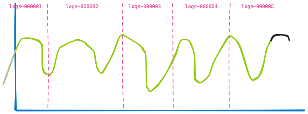
The second visualization is very similar to the first — some data is not shown anymore as it has aged out (left of the blue line) and some more data was added at the end shown in the black line. Can you spot what has not changed? The data returned from indices logs-000002, logs-000003, and logs-000004.
Even if this data had been in the page cache, we still would need to execute the search and the aggregation on top of the results. So, no need to do this double work. In order to make this work, one more optimization has been added to Elasticsearch: the ability to rewrite a query. Instead of specifying a timestamp range for the logs indices logs-000002, logs-000003, and logs-000004, we can rewrite this to a match_all query internally as every document within that index matches with regard to the timestamp (other filters would still apply of course). Using this rewrite, both requests now end up as the exact same request on these three indices and thus can be cached.
This has become the shard-level request cache. The idea is to cache the full response of a request so you do not need to execute any search at all and can basically return the response instantly — as long as the data has not changed to ensure you don’t return any stale data!
Diving deeper
The component responsible for caching is the IndicesRequestCache class. This method is used within the SearchService when executing the query phase. There is also an additional check if a query is eligible for caching — for example, queries that are being profiled are never cached to avoid skewing the results.
This cache is enabled by default, can take up to one percent of the total heap, and can even be configured on a per-request basis if you need to. By default, this cache is enabled for search requests that do not return any hits — exactly what a Kibana visualization request is! However you can also use this cache when hits are returned by enabling it via a request parameter.
You can retrieve statistics about the usage of this cache via:
GET /_nodes/stats/indices/request_cache?human
Summary
The shard-level request cache remembers the full response to a search request and returns those if the same query comes in again without hitting the disk or the page cache. As its name implies, this data structure is tied to the shard containing the data and will also never return stale data.
Query cache
The query cache is the last cache we will take a look at in this post. Again, the way this cache works is rather different to the other caches. The page cache caches data independent of how much of this data is really read from a query. The shard-level query cache caches data when a similar query is used. The query cache is even more granular and can cache data that is reused between different queries.
Let’s take a look how this works. Let’s imagine we search across logs. Three different users might be browsing this month’s data. However, each user uses a different search term:
- User1 searched for “failure”
- User2 searched for “Exception”
- User3 searched for “pcre2_get_error_message”
Every search returns different results, and yet they are within the same time frame. This is where the query cache comes in: it is able to cache just that part of a query. The basic idea is to cache information hitting the disk and only search in those products. Your query is probably looking like this:
GET logs-*/_search
{
  "query": {
    "bool": {
      "must": [
        {
          "match": {
            "message": "pcre2_get_error_message"
          }
        }
      ],
      "filter": [
        {
          "range": {
            "@timestamp": {
              "gte": "2021-02-01",
              "lt": "2021-03-01"
            }
          }
        }
      ]
    }
  }
}
For every query the filter part stays the same. This is a highly simplified view of what the data looks like in an inverted index. Each time stamp is mapped to a document id.
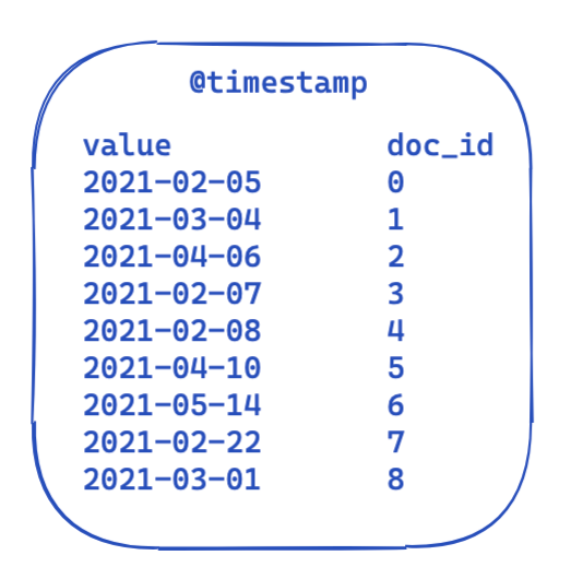
So, how can this be optimized and reused across queries? This is where bit sets (also called bit arrays) come into play. A bit set is basically an array where each bit represents a document. We can create a dedicated bit set for this particular @timestamp filter covering a single month. A 0 means that the document is outside of this range, whereas a 1 means it is inside. The resulting bit set would look like this:
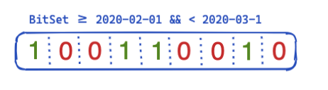
After creating this bit set on a per-segment base (meaning it would need to be recreated after a merge or whenever a new segment gets created), the next query does not need to do any disk access to rule out four documents before even running the filter. Bit sets have a couple of interesting properties. First they can be combined. If you have two filters and two bit sets, you can easily figure the documents where both bits are set — or merge an OR query together. Another interesting aspect of bit sets is compression. You need one bit per document per filter by default. However, by using not fixed bit sets but another implementation like roaring bitmaps you can reduce the memory requirements.
So, how is this implemented in Elasticsearch and Lucene? Let’s take a look!
Diving deeper
Elasticsearch features a IndicesQueryCache class. This class is bound to the lifecycle of the IndicesService, which means this is not a per-index, but a per-node feature — which makes sense, as the cache itself uses the Java heap. That indices query cache takes up two configuration options
- indices.queries.cache.count: The total number of cache entries, defaults to 10,000
- indices.queries.cache.size: the percentage of the Java heap used for this cache, defaults to 10%
In the IndicesQueryCache constructor a new ElasticsearchLRUQueryCache is set up. This cache extends from the Lucene LRUQueryCache class. That class has the following constructor:
 public LRUQueryCache(int maxSize, long maxRamBytesUsed) {
    this(maxSize, maxRamBytesUsed, new MinSegmentSizePredicate(10000, .03f), 250);
  }
The MinSegmentSizePredicate ensures that only segments with at least 10,000 documents are eligible for caching and have more than 3% of the total documents of this shard.
However, things are a little bit more complex from here. Even though the data is in the JVM heap, there is another mechanism that tracks the most common query parts and only puts those into that cache. This tracking, however, happens on the shard level. There is a UsageTrackingQueryCachingPolicy class that uses a FrequencyTrackingRingBuffer (implemented using fixed-size integer arrays). This caching policy also has additional rules in its shouldNeverCache method, which prevents caching of certain queries like term queries, match all/no docs queries, or empty queries, as these are fast enough without caching. There is also a condition for the minimum frequency to be eligible for caching, so that a single invocation will not result in the cache being filled. You can track use, cache hit rates and other information via:
GET /_nodes/stats/indices/query_cache?human
Summary
The query cache gets on the next granular level and can be reused across queries! With its built-in heuristics it only caches filters that are used several times and also decides based on the filter if it is worth caching or if the existing ways to query are fast enough to avoid wasting any heap memory. The lifecycle of those bit sets is bound to the lifecycle of a segment to prevent returning stale data. Once a new segment is in use, a new bit set needs to be created.
Are caches the only possibility to speed things up?
It depends (you already guessed that this answer had to come up in this blog at some point, right?). A recent development in the Linux kernel is rather promising: io_uring. This is a new way of doing asynchronous I/O under Linux using completion queues available since Linux 5.1. Note that io_uring is still in heavy development. However, there are first tries in the Java world to use io_uring like netty. Performance tests for simple applications look stunning. I guess we have to wait a bit until we see real-world performance numbers, even though I expect those will have significant changes as well. Let’s hope that support for this will at some point be available within the JDK as well. There are plans to support io_uring as part of Project Loom, which might bring io_uring to the JVM. More optimizations like being able to hint the access pattern to the Linux kernel via madvise() are also not yet exposed in the JVM. This hint prevents a read-ahead issue, where the kernel tries to read more data than is needed in anticipation of the next read, which is useless when random access is required.
That's not all! The Lucene developers are busy as always to get the most out of any system. There is a first draft of a rewrite of the Lucene MMapDirectory using the Foreign Memory API, which might become a preview feature in Java 16. However, this was not done for performance reasons, but to overcome certain limitations with the current MMap implementation.
Another recent change in Lucene was getting rid of native extensions by using direct i/o (O_DIRECT) in the FileChannel class. This means that writing data will not thrash the page cache — this will be a Lucene 9 feature.
Sometimes you can also speed things up so that you probably don’t even have to think about a cache anymore, reducing your operational complexity. Recently there was a huge improvement of speeding up date_histogram aggregations several times. Take your time and read that long but enlightening blog post.
Another very good example of a tremendous improvement (without caching) was the implementation of block-max WAND in Elasticsearch 7.0. You can read all about it in this blog post by Adrien Grand.
Wrapping up the caching deep dive
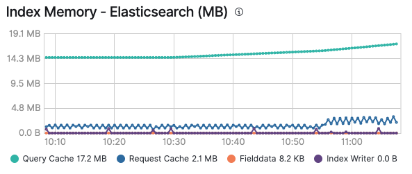
I hope you enjoyed the ride across the various caches, and now got a grasp when which cache will kick in when. Also keep in mind that monitoring your caches can be especially useful to figure out whether a cache makes sense or keeps getting thrashed due to constant addition and expiration. Once you enable monitoring of your Elastic cluster, you can see memory consumption of the query cache and the request cache in the Advanced tab of a node, as well as on a per-index base, if you look at a certain index:
All of the existing solutions on top of the Elastic Stack will make use of these caches to make sure to execute queries and deliver your data as fast as possible. Remember that you can enable logging and monitoring in Elastic Cloud with a single click and have all your clusters monitored at no additional cost. Try it out yourself or explore ways to speed up query performance in this webinar.