The impact of absolute values vs. percentages on effective machine learning
Overcoming machine learning model imperfections to detect anomalies in online chess games


 Share on Twitter
Share on Twitter

 Share on LinkedIn
Share on LinkedIn

 Share on Facebook
Share on Facebook

 Share by Email
Share by Email

 Print this page
Print
This is the fourth blog post in our chess series (don’t forget to check out the first, second, and third posts!). Chess is a fascinating game. What can happen on those 64 squares?
Lichess is a platform that allows you to play chess; it publishes all rated games as archives, starting in 2013. There are a total of over 4 billion games played. Yes, 4 billion matches.
In the third blog, we analyzed the impact of chess YouTubers and streamers such as GothamChess and Hikaru Nakamura and showed how to calculate the significance. What about our machine learning capabilities? Would our machine learning models, especially anomaly detection, detect the increase as an anomaly?
The first model
A straightforward machine learning model that counts the records of played games with the Ponziani opening should do the trick.
- Head over to discover type `opening.name: *Ponziani*` in the search bar. Save this search.
- Go to machine learning, select anomaly detection, create a new job, and select the saved search.
- In the single metric option, select Count. We just want to know how many games played this opening. Depending on how granular you want your model, you can choose between one day and seven days or even more for the bucket size. I tend to do seven days since we are talking about 10+ years worth of chess data, and I am more interested in long-lasting changes than just a daily fluke.
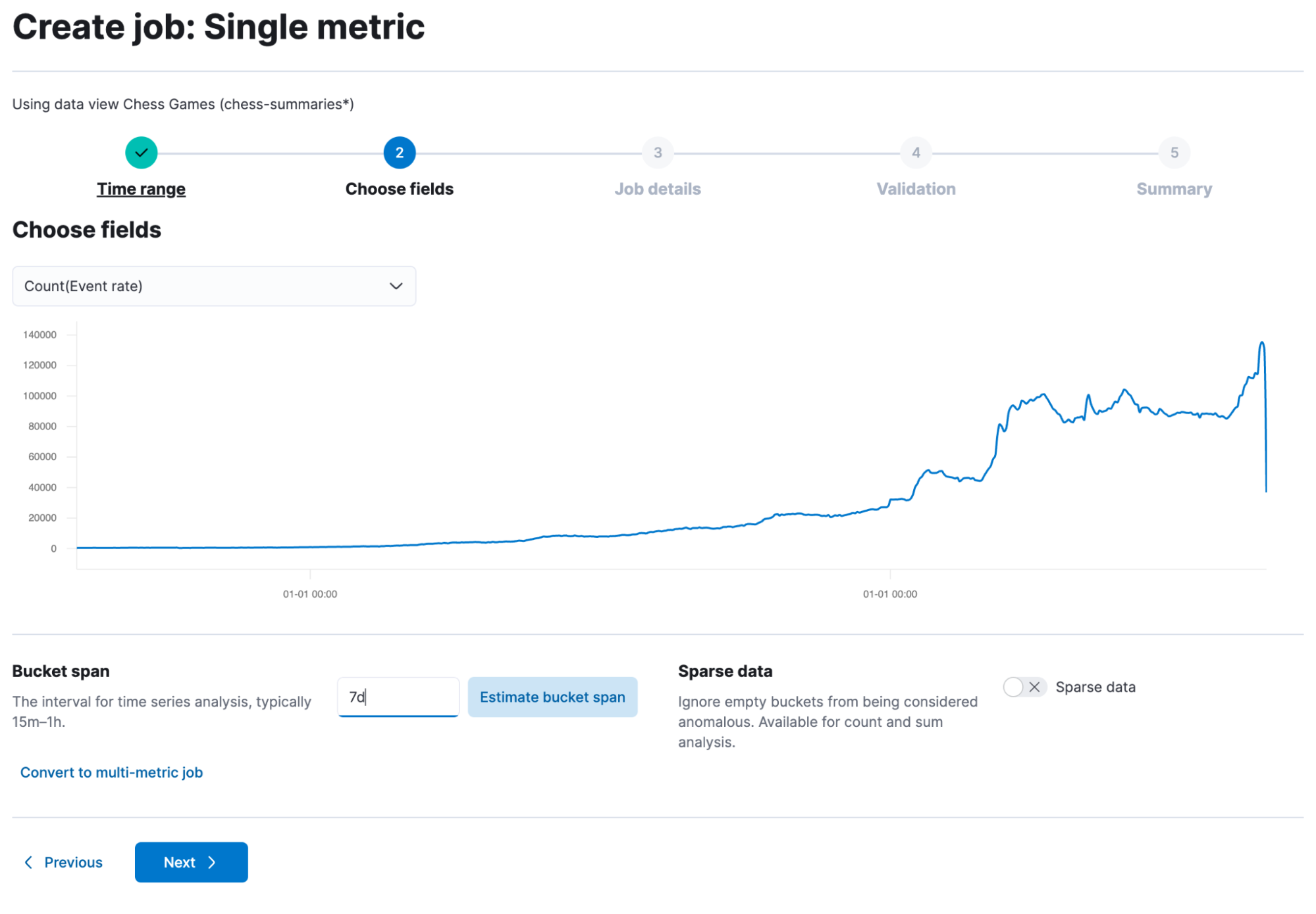
Then click through the UI, give it a name, and start it. Once it is finished, you will be able to view the results!
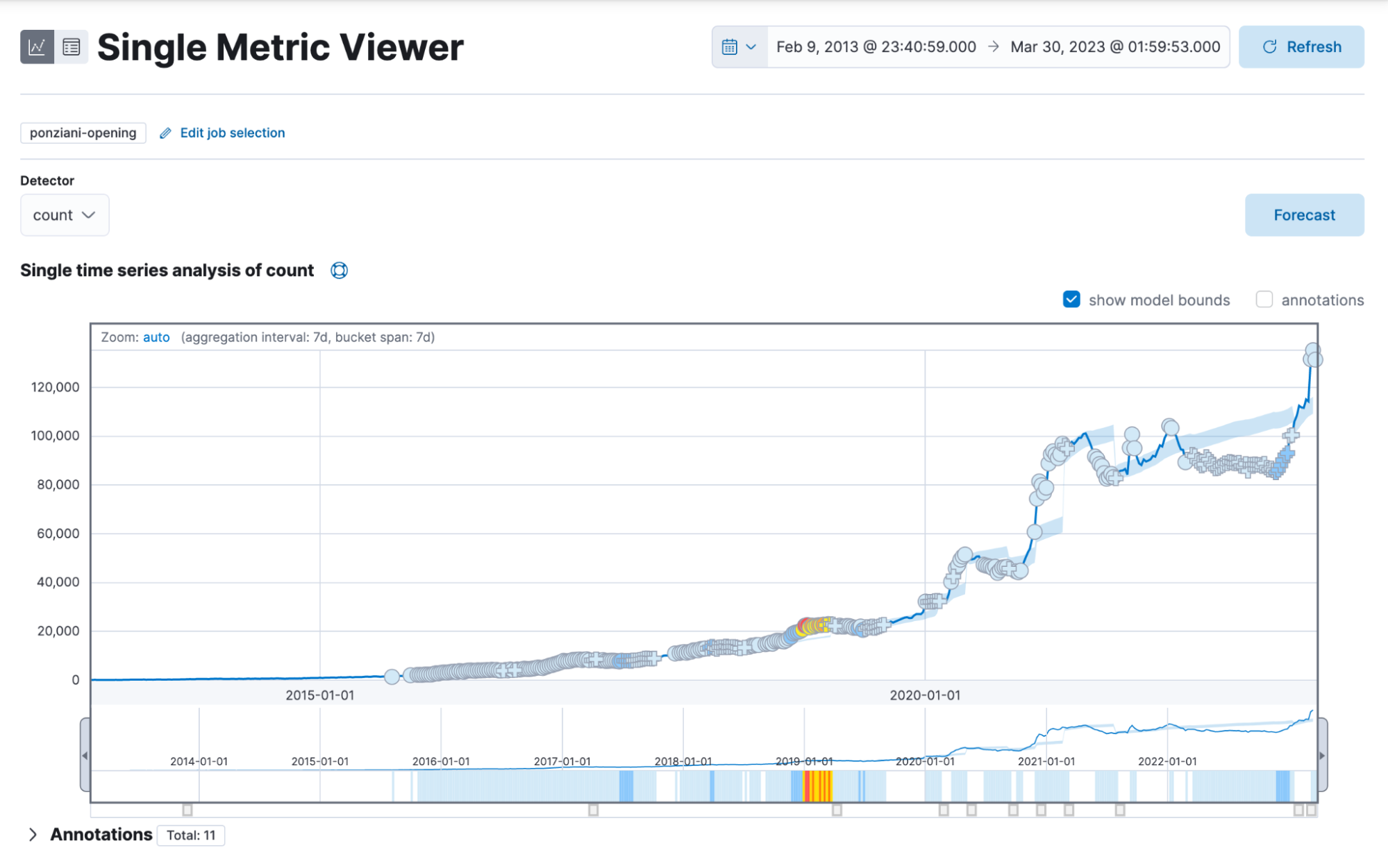
Those results look engaging. As we can see, there are a lot of situations where the model detects an anomaly (marked by crosses and circles). The shaded area around the blue line is the model bounds, which is the area where your model thinks the following data should be. The blue line is the actual value. I don’t enjoy this view that much, as there are many anomalies just because there is a generally steady rising trend in the number of games played, which leads to confusion. How can we resolve this? Instead of relying on absolute values, we could use percentages.
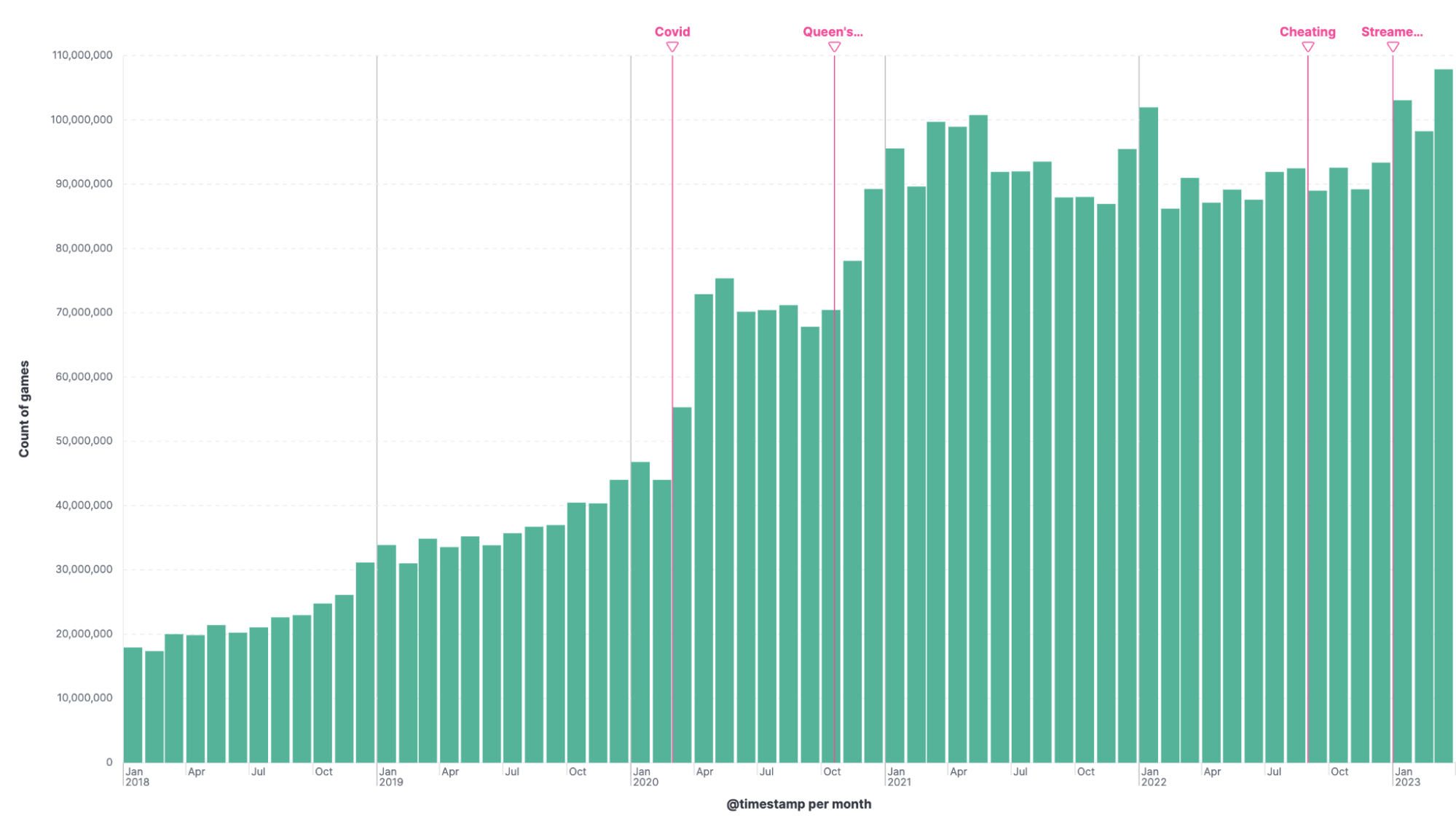
Checking back in a quick Lens visualization that displays all games played on the Lichess Plattform shows a steady upward trend:
- A spike in 2020, around March and April, correlates with the coronavirus pandemic and more people being at home with time to play chess, particularly online with friends. The games played were reduced as soon as the summer months hit and the lockdowns and other restrictions were largely lifted.
- In October 2020 “The Queen’s Gambit” a popular Netflix show, was released.
- In September 2022, there was the Carlsen-Niemann controversy.
- In January 2023, multiple Youtubers and streamers had a massive surge in subscribers and thus viewer counts of videos.
The short dip in February can be explained because it is missing two full days (only 28 days long as opposed to January 31 and March 30). January has 103 million games, February 98 million, and March 108 million.
The second model and data feed
What can we now change with the first model to identify the anomalies better? When going for total values, as in “how many games were played with the Ponziani opening” like in our first model, you are not only looking at the count of Ponzianis played, but the total number of games automatically sways the model, since it is only possible to have more Ponzianis when there are more games.
Inadvertently, the first model automatically detects the general playing trend as well. Calculating the percentage of games played with the Ponziani might be more appropriate to circumvent this. We can calculate this using a pivot transform (explained more in-depth in this blog) or the data feed to calculate the percentage. We will use the Advanced Model creation UI inside Kibana Machine Learning for this.
On the second page, click edit JSON to get a flyout. Inside the Datafeed Configuration JSON, add this. First, we query all data, which is what the match_all is doing for us. We only use indices that have the chess-summaries alias.
Inside the aggregations, we create daily buckets; we need to have a max aggregation, so the highest value is inside this daily bucket. We then do a value_count, which translates to “count all documents containing that field” and gives us all games played on that day. Last but not least, we create a filter aggregation that tells us how many Ponzianis are played. Then it is just a simple bucket script to calculate the percentage of Ponzianis.
{
  "query": {
    "match_all": {}
  },
  "indices": [
    "chess-summaries*"
  ],
  "aggregations": {
    "buckets": {
      "date_histogram": {
        "field": "@timestamp",
        "fixed_interval": "1d"
      },
      "aggregations": {
        "@timestamp": {
          "max": {
            "field": "@timestamp"
          }
        },
        "count": {
          "value_count": {
            "field": "opening.name"
          }
        },
        "ponziani": {
          "filter": {
            "bool": {
              "filter": [
                {
                  "wildcard": {
                    "opening.name": {
                      "value": "*Ponziani*"
                    }
                  }
                }
              ]
            }
          }
        },
        "percent": {
          "bucket_script": {
            "buckets_path": {
              "total": "count",
              "ponz": "ponziani>_count"
            },
            "script": "params.ponz/params.total"
          }
        }
      }
    }
  },
  "scroll_size": 1000,
  "delayed_data_check_config": {
    "enabled": true
  },
  "job_id": "",
  "datafeed_id": "datafeed-"
}Now that this is in place, you also need to add a detector and so on. This is done in the Job Configuration JSON. This is the detector, and you need to add a summary_count_field_name.
  "summary_count_field_name": "doc_count",
    "detectors": [
      {
        "function": "max",
        "field_name": "percent",
        "detector_description": "max(percent)"
      }
],All in all, in the end, it should look similar to this:
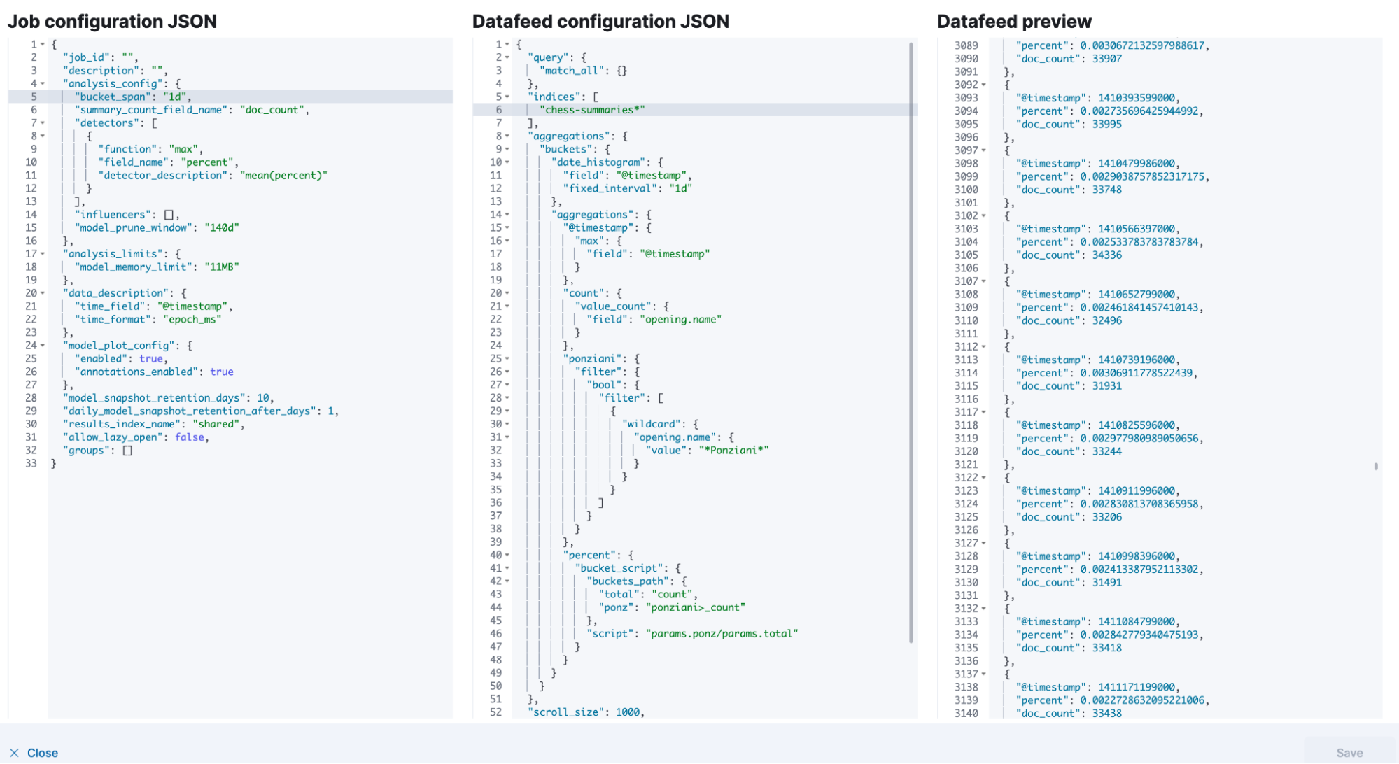
Click on Save and go through the rest of the guided setup. Start the machine learning job and wait until it’s finished. Let’s go to the Single Metric viewer and plot it.
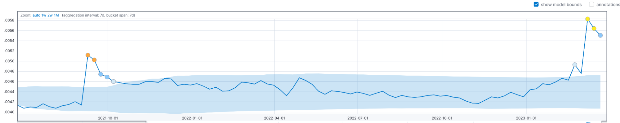
We get a better-fitted model. From left to right, we got some anomalies in September 2021. It could well be that this aligns nicely with a Ponziani Opening Tutorial from Eric Rosen published on 11 September of that year. When we go to the right, we get the anomalies in March, as expected due to the GothamChess Youtube Tutorial.
Summary
This blog post showed the difference the value used for a machine learning model can have on its effectiveness. Total values, percentages, and logarithmic scales can all solve various problems and ensure that your anomaly detection performs the best job.
Ready to get started? Begin a free 14-day trial of Elastic Cloud. Or download the self-managed version of the Elastic Stack for free.
Share
- Share on Twitter
Share on Twitter
- Share on LinkedIn
Share on LinkedIn
- Share on Facebook
Share on Facebook
- Share by Email
Share by Email
- Print this page
Print