Follow the money: tracing laundering networks with ES|QL and cross-cluster search
The data model, cross-cluster architecture and five ES|QL queries that power mule detection and laundering network tracing, built from infrastructure most financial institutions already run.
Five ES|QL queries flag money mule accounts across an entire portfolio, trace laundering networks downstream from a single reported case, and correlate suspicious payments against behavioral signals in a separate cluster without moving any data. This post covers the architecture, data model and ES|QL queries behind the fraud investigation platform we built on Elasticsearch.. It also covers how tiered storage and logsdb index mode bring seven-year regulatory retention costs down by up to 65%. Part 2 of three; Part 1 covered the investigation gap in financial services, Part 3 will cover the AI agents built on top.
How the fraud investigation platform came together
We demonstrated this platform at a recent UK Customer Tech Talk. The key point worth emphasizing: Elasticsearch, Agent Builder, ES|QL, and Kibana are components many financial institutions already run, so the investigation capability described here can be assembled from existing infrastructure rather than purchased as a separate stack.
Fraud investigation platform architecture on Elasticsearch
The platform follows a layered architecture with clear separation between data, intelligence, and presentation.
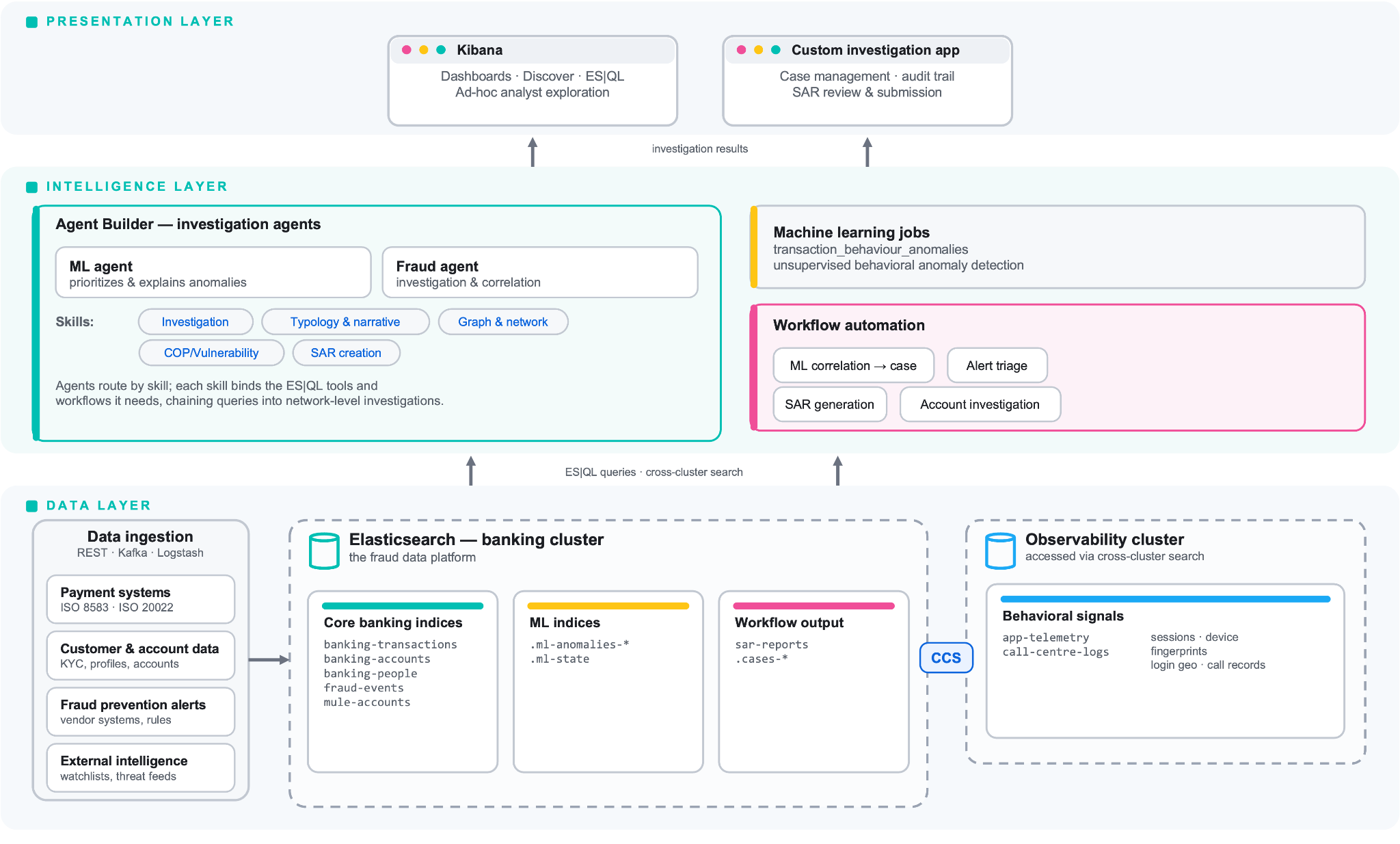
Fig 1. High-level Elastic Architecture
Data layer: two clusters, one search
Fraud investigation data rarely lives in one place. Transaction records, customer profiles, and account metadata typically sit in a banking data cluster managed by payments or core banking teams. Meanwhile, application telemetry (mobile app session logs, online banking events, device fingerprints, and call center interaction records) often lives in an observability cluster managed by engineering or operations teams.
Cross-cluster search (CCS) allows each team to keep ownership of its data. At the same time, investigators can query across both clusters in a single request without migrating into a single cluster and without a separate aggregation layer. The banking cluster holds transactional data; the observability cluster holds behavioral signals. Investigators see one unified result set without either team giving up control of their data.
Cross-cluster search is not just a technical convenience. It addresses the intra-organisational barriers we described in Part 1 - different teams owning different data, concerns about query impact on production systems, and role-based access controls that exist for good reason. CCS respects all of these while still allowing cross-domain investigation.
Intelligence layer: Agent Builder, skills, and workflows
The intelligence layer is where AI agents, ES|QL queries, machine learning jobs, and workflow automation come together. In Elastic Agent Builder, agents route a request to the right skill, and each skill binds the ES|QL tools and workflows it needs; for example, Investigation, Typology & Narrative, Graph & Network, COP/Vulnerability, and SAR Creation. Part 3 covers the agent and skill architecture in detail. In this blog, we focus on the data and query foundations they depend on.
Presentation layer: Kibana and custom applications
The platform includes a custom investigation interface that communicates with the agent service and Elasticsearch APIs. But the same data is also available in Kibana for ad-hoc, analyst-driven exploration. This dual-interface approach is intentional: structured investigation workflows for speed, and Kibana for questions the workflow was not designed to answer.
Kibana dashboards provide operational views (alert queues, case volume trends, and mule account heatmaps), while Discover and ES|QL in the console give analysts the freedom to run exploratory queries without waiting for someone to build a new dashboard.
A note on availability: the data model and ES|QL queries shown here run on any Elasticsearch deployment, but two capabilities in this architecture have specific requirements:
Cross-cluster search with ES|QL is generally available in Elasticsearch 8.19 and 9.1; requires a compatible subscription on both clusters (see cross-cluster search and subscriptions).
Elastic Agent Builder is available on Elastic Cloud Serverless and on the Enterprise tier for cloud-hosted and self-managed deployments (see Agent Builder general availability).
Data model for money mule detection: transactions, accounts and behavioral signals
The data model is the foundation of everything else. Fraud investigation is a cross-domain problem, which means the data model must accommodate different document types while still supporting fast, flexible querying.
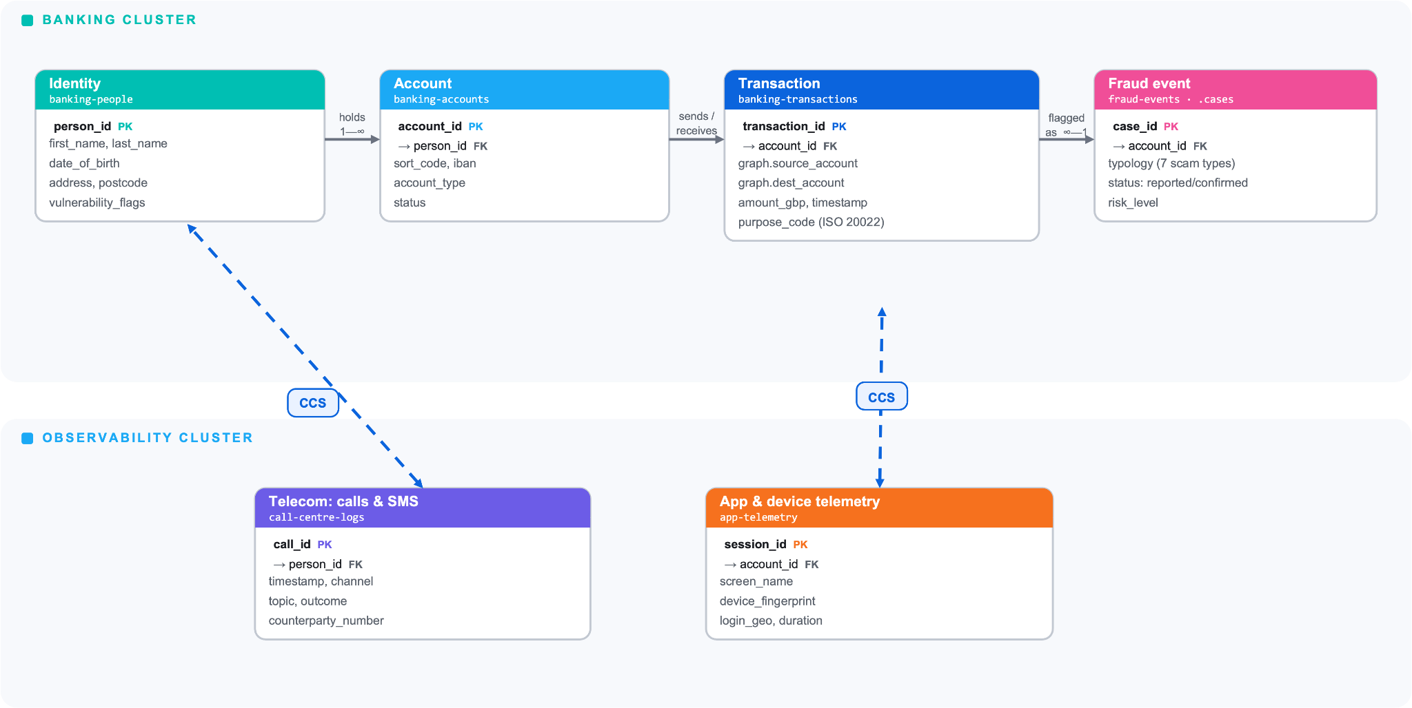
Fig 2. App Fraud Data Model - FCA Sandbox
Banking transactions
The core index holds payment transaction records. Each document represents a single payment event with fields for the parties involved, amounts, timing, and metadata.
// Index: banking-transactions
{
  "transaction_id": "a76fe1f9-c403-4855-bc61-22b0db37fc29",
  "timestamp": "2025-01-20T23:47:12.341Z",
  "account_id": "3f7932e3-9e69-4d69-aef5-41f281b3969b",
  "amount_gbp": -15000,
  "currency": "GBP",
  "is_credit": false,
  "is_debit": true,
  "channel": "mobile_app",
  "transaction_type": "faster_payment",
  "payment_code": "XF",
  "purpose_code": "INVESTMENT",
  "description": "Investment deposit",
  "counterparty_name": "CryptoTrade Ltd",
  "counterparty_account": "94738291",
  "counterparty_sort_code": "20-45-67",
  "merchant_category": "6211",
  "geo_location": "POINT (-0.1616 51.5296)",
  "graph.source_account": "47-83-82_10985194",
  "graph.source_bank": "Bank4",
  "graph.dest_account": "20-45-67_94738291",
  "graph.dest_bank": "Bank2",
  "graph.payment_flow": "outbound",
  "graph.amount_band": "large",
  ...
}
A few things stand out about this structure.
The
purpose_codeandmerchant_categoryfields carry ISO 20022 enrichment where available, providing signals that a rules-based system can use alongside the AI agent.Negative amounts denote debits, with
is_creditandis_debit flagsfor fast filtering.geo_locationenables spatial analysis of transaction patterns.
Where ISO 20022 enriched data is available, purpose codes, Legal Entity Identifiers, and structured remittance information provide additional signals. The schema-agnostic nature of Elasticsearch means we can ingest both ISO 8583 legacy formats and ISO 20022 enriched formats into the same index without a rigid upfront schema.
Accounts and people
Customer data is generally hosted in a CDP (Customer Data Platform), but to simplify the architecture, we put it in the same cluster. Account-level data is in a banking-accounts index, while customer identity and profile data live in banking-people. This separation is deliberate: investigators who need to query transaction patterns can do so without accessing personally identifiable information, and RBAC controls can restrict PII access to authorised roles.
// Index: banking-accounts
{
  "account_id": "7179a225-19b5-4b24-9aae-b50ad43cb15c",
  "account_number": "96435152",
  "account_type": "savings_account",
  "account_status": "active",
  "person_id": "79393ff4-3a32-4bae-9021-4566e6b5008c",
  "bank_name": "Bank1",
  "sort_code": "20-30-79",
  "iban": "GB62BANK20307996435152",
  "balance_gbp": 39920.61,
  "currency": "GBP",
  "opened_date": "2017-04-13T00:00:00.000Z",
  ...
}
The person_id field links to the banking-people index, which holds customer identity, address, credit history, employment, and vulnerability flags (kept in a separate index with its own access controls). A simplified example:
// Index: banking-people
{
  "person_id": "4233d7fd-29aa-439d-8cc8-a07f1933128f",
  "first_name": "Rebecca",
  "last_name": "Brennan",
  "date_of_birth": "1979-01-19T00:00:00.000Z",
  "age": 47,
  "address_line1": "244 Manor Terrace",
  "city": "Blackpool",
  "postcode": "FY1 6AN",
  "location_geo": "POINT (-3.050282 53.836826)",
  "credit_history.credit_score": 729,
  "credit_history.vulnerability_flag": "socially_isolated",
  "credit_history.total_debt_gbp": 6548.49,
  "accounts": [
    { "account_id": "528a...", "account_number": "32540475",
      "sort_code": "22-79-61", "balance_gbp": 3242.93 },
    { "account_id": "692e...", "account_number": "39261497",
      "sort_code": "24-53-93", "balance_gbp": 2175.45 }
  ],
  ...
}
Application telemetry (observability cluster)
The observability cluster holds session-level telemetry from the bank’s own mobile and online banking applications. This is not browsing history or external website data. It is telemetry from the institution’s own services, which payment service providers legitimately have access to.
// Index: app-telemetry (observability cluster, accessed via CCS)
{
  "session_id": "sess-9f8e7d",
  "customer_id": "C847392",
  "timestamp": "2025-01-20T21:32:00Z",
  "app_platform": "ios",
  "event_type": "screen_view",
  "screen_name": "payment_limits",
  "session_duration_seconds": 8100,
  "device_fingerprint": "fp-abc123",
  "ip_address": "82.132.xxx.xxx",
  "geo_city": "London",
  ...
}
Session telemetry reveals behavioral patterns that transaction data alone cannot: how long a customer spends in the app before making a payment, which screens they visit (particularly payment limit screens), whether the device fingerprint matches their normal device, and whether the login location is consistent with their history.
Call center logs
Customer service interactions are indexed with structured metadata, making it possible to correlate service calls with subsequent transactions.
// Index: call-centre-logs
{
  "call_id": "CALL-29481",
  "customer_id": "C847392",
  "timestamp": "2025-01-17T14:22:00Z",
  "duration_seconds": 420,
  "topic": "payment_limit_increase",
  "outcome": "limit_raised",
  ...
}
How do you detect money mule accounts with ES|QL?
ES|QL is Elastic’s piped query language, designed for exploratory analysis across large datasets. In our platform, ES|QL queries serve two roles: they are the tools that agent skills invoke programmatically, and they are available directly to analysts in Kibana for ad-hoc exploration.
Here are the key queries that power the platform.
Mule detection: finding accounts where money flows straight through
This is the most important query in the platform. It looks at every account, calculates how much money came in versus how much went out, measures how quickly that happened, and flags the accounts where money is flowing straight through.
FROM banking-transactions
| STATS
    incoming = SUM(CASE(is_credit == true, amount_gbp, 0)),
    outgoing = SUM(CASE(is_debit == true, ABS(amount_gbp), 0)),
    transaction_count = COUNT(*),
    first_txn = MIN(timestamp),
    last_txn = MAX(timestamp)
  BY account_id
| EVAL
    turnover_ratio = TO_DOUBLE(outgoing) / GREATEST(TO_DOUBLE(incoming), 1.0),
    time_span_ms = TO_LONG(last_txn) - TO_LONG(first_txn),
    days_active = time_span_ms / 86400000.0,
    txn_frequency = TO_DOUBLE(transaction_count) / GREATEST(days_active, 1.0)
| WHERE incoming > 5000
    AND turnover_ratio > 0.75
    AND days_active < 180
| SORT turnover_ratio DESC, incoming DESC
| LIMIT 50
Sample output:
account_id         incoming  outgoing  txns  turnover_ratio  days_active
20-45-67_94738291   247,000   239,000    31           0.968         42.0
30-91-22_50271841    87,000    84,200    18           0.968         27.0
04-17-55_61398002    54,000    52,400    13           0.970         22.0
11-38-09_77450513    43,000    41,500    11           0.965         18.0

(top 4 of 50 results)
A turnover_ratio close to 1.0 means almost everything that came in went straight back out; the hallmark of a mule account. The days_active filter focuses on recently opened accounts, and the incoming threshold filters out noise. The result is a ranked list of the most suspicious accounts in the portfolio.
Profiling a suspect account: who is sending money in?
Once an account is flagged, the next step is understanding the inbound pattern. This query identifies every account that sent money to a given destination and calculates the total exposure per source.
FROM banking-transactions
| WHERE graph.dest_account == "20-45-67_94738291"
    AND is_debit == true
| STATS
    total_sent = SUM(ABS(amount_gbp)),
    tx_count = COUNT(*),
    first_payment = MIN(timestamp),
    last_payment = MAX(timestamp)
  BY graph.source_account, graph.source_bank
| SORT total_sent DESC
Sample output:
graph.source_account  graph.source_bank  total_sent  tx_count
20-30-79_88142251     Bank1                  15,000         1
04-22-13_67391044     Bank3                  14,200         1
11-90-56_20517783     Bank2                  12,800         2
...                   ...                       ...       ...

23 source accounts · £247,000 total
This surfaces the full list of source accounts - the potential victims. When an account shows 23 distinct sources over six weeks, all sending large sums to the same destination, the pattern is clear.
Tracing the network downstream
Mule networks are layered. To trace where the money goes after the primary mule, we flip the query to look at outbound flows:
FROM banking-transactions
| WHERE graph.source_account == "20-45-67_94738291"
    AND graph.payment_flow == "outbound"
| STATS
    forwarded = SUM(ABS(amount_gbp)),
    tx_count = COUNT(*),
    first_forward = MIN(timestamp),
    last_forward = MAX(timestamp)
  BY graph.dest_account, graph.dest_bank
| SORT forwarded DESC
Sample output:
graph.dest_account  graph.dest_bank  forwarded  tx_count
30-91-22_50271841   Bank4              112,400         8
04-17-55_61398002   Bank2               78,100         6
11-38-09_77450513   Bank5               48,500         4

3 downstream accounts · £239,000 forwarded
The agent chains these queries together: profiling the primary mule’s downstream accounts, then running the same mule detection query against each of them to assess whether they are also part of the laundering network. This recursive pattern is what turns a single reported case into a full network-level investigation.
Customer behavioral baseline
To assess whether a specific transaction is unusual for a given customer, we calculate their historical baseline and compare:
FROM banking-transactions
| WHERE account_id == "3f7932e3-9e69-4d69-aef5-41f281b3969b"
    AND is_debit == true
| STATS
    avg_amount = AVG(ABS(amount_gbp)),
    max_amount = MAX(ABS(amount_gbp)),
    tx_count = COUNT(*),
    first_txn = MIN(timestamp),
    last_txn = MAX(timestamp)
| EVAL
    flagged_amount = 15000,
    amount_ratio = ROUND(flagged_amount / GREATEST(avg_amount, 1.0), 1),
    time_span_ms = TO_LONG(last_txn) - TO_LONG(first_txn),
    days_active = time_span_ms / 86400000.0
Sample output:
avg_amount  max_amount  tx_count  flagged_amount  amount_ratio  days_active
  1,247.50    4,200.00        87          15,000          12.0        363.8
An amount_ratio of 12 means the flagged transaction is 12 times the customer’s typical payment. The agent uses this, alongside timing and channel data, as input to its fraud likelihood assessment.
Cross-cluster behavioral context
Cross-cluster search allows a single ES|QL query to pull data from the observability cluster. This query retrieves the customer’s app telemetry in the hours leading up to the flagged transaction:
FROM observability:app-telemetry
| WHERE account_id == "3f7932e3-9e69-4d69-aef5-41f281b3969b"
    AND timestamp >= "2025-01-20T19:00:00Z"
    AND timestamp <= "2025-01-21T00:00:00Z"
| STATS
    session_count = COUNT_DISTINCT(session_id),
    total_duration = SUM(session_duration_seconds),
    screens_viewed = COUNT(*),
    limit_views = SUM(CASE(screen_name == "payment_limits", 1, 0))
| EVAL hours_active = ROUND(TO_DOUBLE(total_duration) / 3600.0, 1)
Sample output:
session_count  total_duration  screens_viewed  limit_views  hours_active
            4           7,320              38            7           2.0
When this reveals that a customer who normally spends five minutes banking at lunchtime instead spent two hours in the app late at night, visited the payment limits screen seven times, and then made an unusually large transfer, the picture becomes much clearer. This behavioral context is often the difference between a confident fraud assessment and an ambiguous one.
Scaling fraud data retention with Elasticsearch tiered storage
A fraud investigation platform is only useful if it can handle real-world data volumes and regulatory retention requirements.
Data volumes
Elasticsearch’s distributed architecture handles this comfortably. The same infrastructure that processes billions of security events daily for enterprise customers is more than capable of handling payment transaction volumes (customers such as BBVA).
Tiered storage for regulatory retention
UK financial regulations typically require seven years of transaction data retention. That is a lot of data. Elastic’s tiered storage architecture makes this economically viable:
Hot tier (NVMe SSDs): The last 7 to 30 days. Sub-second query performance for active investigations and real-time alerting.
Warm tier (SSDs): 30 days to one year. Fast enough for historical case review and pattern analysis.
Cold tier and frozen tier (object storage): One to seven years. Compliance and audit queries, training data for ML models.
Logsdb for cost reduction
Logsdb index mode reduces storage costs by up to 65% for transaction data by optimizing how fields are stored and indexed. For a platform retaining years of data at scale, this is the difference between an affordable deployment and a prohibitively expensive one.
Key lessons building a fraud investigation platform on Elasticsearch
Building the Elasticsearch fraud investigation platform reinforced a few lessons worth sharing for anyone building something similar.
Lesson | Why it matters | What to do |
|---|---|---|
Start with the data model | A well-defined schema gives AI agents the context to interpret query results accurately. Every downstream query, skill and dashboard depends on it. | Define explicit mappings upfront, e.g. field names, types and relationships. Normalise field names across indices, define clear document boundaries, and plan for cross-cluster query patterns. |
Behavioral data is the differentiator | Transaction data alone is ambiguous. A £15,000 payment to an unfamiliar account could be a house deposit, a car purchase or fraud. Behavioral context (e.g. two hours of app usage at midnight, seven visits to the payment limits screen, a call center request three days prior) is what turns ambiguity into confidence. | Ingest app session telemetry alongside transaction data and query it via cross-cluster search at investigation time. |
Cross-cluster search makes the architecture realistic | CCS allows investigators to query across banking and observability clusters while respecting existing data ownership boundaries. Without it, you need data migration or a separate aggregation layer. | Treat CCS as a structural requirement, not an optimisation. It is what makes this architecture deployable in a real institution. |
Next: AI agents and workflow automation
With the data model and query foundations in place, part 3 will cover the AI agents built on top of this architecture: how they are configured, which tools they use, how workflow automation handles SAR report generation and account investigation, and a worked scenario that demonstrates the complete investigation flow from alert to compliance action. The result is a unified, queryable investigation layer built from infrastructure that many institutions already run.
Ready to explore Elastic for fraud investigation? Talk to our financial services team about a proof of concept with your data, an architecture review of your current fraud stack, or a strategic discussion on how Elastic fits your fraud roadmap.