AI video search with Elasticsearch and Jina: Find the exact seconds of footage you need

Try out vector search for yourself using this self-paced hands-on learning for Search AI. You can start a free cloud trial or try Elastic on your local machine now.

Type warm sunset light over a mountain, and get back the exact seconds of footage that match. Omnishot is an AI video search app that watches a folder and cuts each clip at its scene boundaries. It embeds every scene as a 1,024-dimension vector with jina-embeddings-v5-omni-small. One model handles both text and video, so a typed query and a piece of footage land in the same vector space, and a nearest neighbor search in Elasticsearch finds the clips that look like the description. An hour of footage becomes about 1,200 searchable vectors, and a folder that used to take hours to ingest goes through in minutes.

The idea came from a video editor here at Elastic. She was losing whole afternoons scrubbing through B-roll folders to find one specific visual.

Searching a footage library by description

Here's what the app does:

1. Select a folder of footage.

2. Search for clips with a visual query (drone shot over a coastline).

3. Search for similar clips using stored vectors.

4. Find similar chunks within the same clip.

5. Reveal the clip in your file browser, ready to drop on a timeline.

How the AI video search pipeline works

The pipeline is as follows:

1. A watcher polls the linked library folder (clips/ by default) every four seconds for new footage. 

2. PySceneDetect detects the scene boundaries in each clip. 

3. FFmpeg cuts the clip at those boundaries with a lossless stream copy and then transcodes each scene chunk into a small proxy. 

4. The proxy goes to jina-embeddings-v5-omni-small through the Jina API, which samples 32 frames and returns a 1,024-dimension vector. 

5. That vector is ingested into Elasticsearch in a dense_vector field with a hierarchical navigable small world (HNSW) index (an approximate nearest neighbor graph). At query time, the editor's text runs through the same model and we do a k-nearest neighbor (kNN) search against the stored chunk vectors.

The same model embeds both text and video, which is what makes Jina’s omni model so versatile. Video chunks and text queries are embedded into the same vector space, so a nearest-neighbor search effectively means find the footage that looks like what I described in text.

What you need to build AI video search

• Elasticsearch (Serverless or 8.x+ with dense vector support)

• A Jina API key

• PySceneDetect

• FFmpeg

• Python 3.9+

Downloading sample footage to search

If you don’t have any footage handy to search through, the repo includes two download scripts: one for short stock clips from the Pexels API, across categories like nature, urban, animals, and more. The other uses yt-dlp to grab longer documentary-style videos directly from YouTube.

python scripts/download_pexels.py --out ./clips --total 50
python scripts/download_youtube.py --out ./clips --total 20

We’re aiming to have a good mix between short and long videos to demonstrate how important the chunking strategy becomes. We’ll discuss that in the next part.

How to chunk video for embeddings

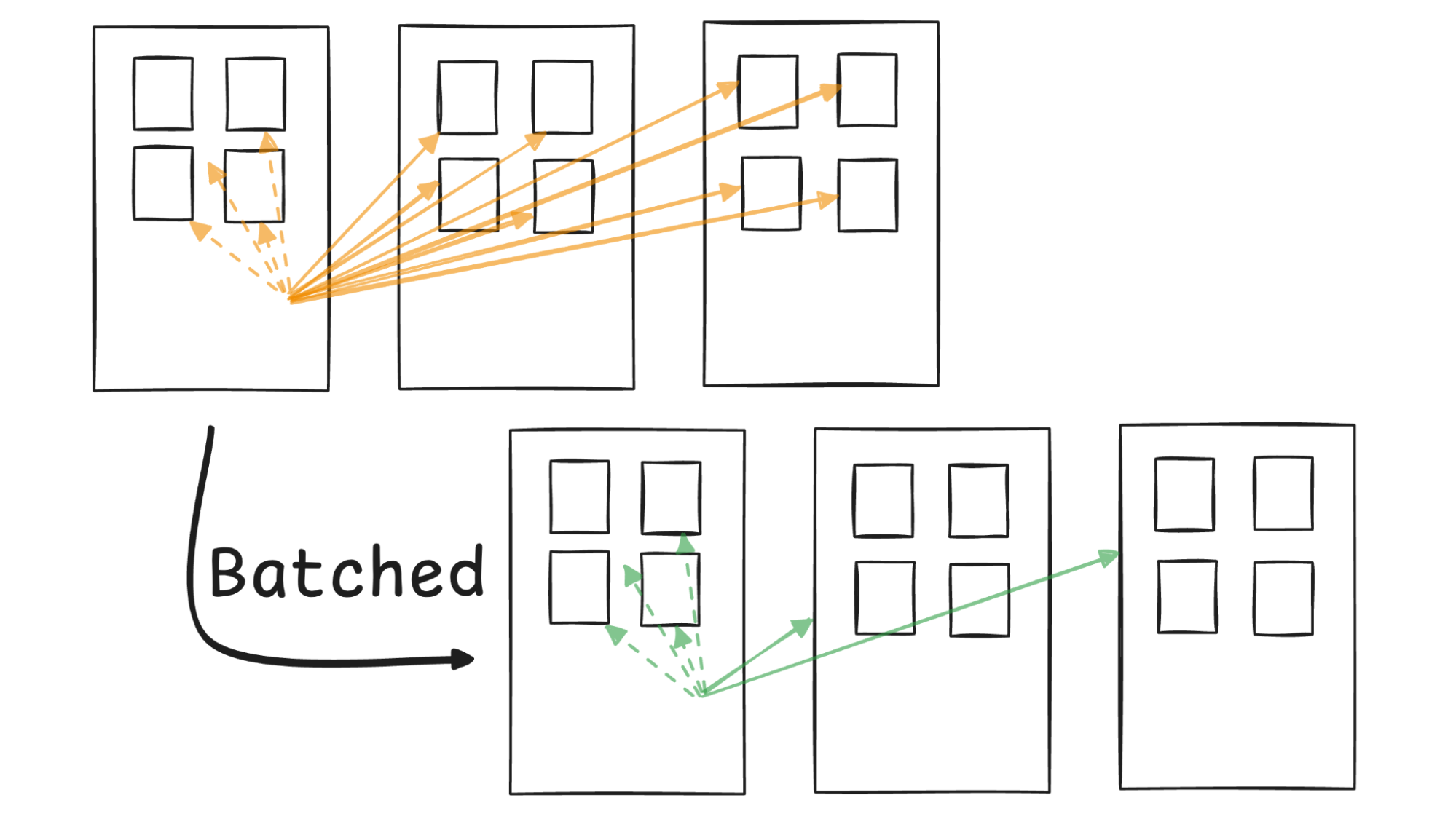
jina-embeddings-v5-omni-small samples 32 evenly spaced frames from whatever video you send it. For a 10-second clip, 32 frames is dense coverage; almost every moment gets captured. For a 10-minute documentary, those same 32 frames are spread so thin that entire shots can be missed. Here’s a diagram illustrating how the Jina model samples each video clip and the limitations with longer clips:

So before we embed anything, we chunk. The question is where to cut. Here's a diagram comparing three strategies:

1. Fixed-length chunking splits every N seconds. It’s simple and predictable, but the cuts can land mid-shot. You could end up with a chunk that’s half drone shot and half talking head, which can make your search results unusable. This isn’t the right fit for this use case.
2. Transcript-based chunking first runs speech to text over the clip to generate a transcript and then applies a text chunking technique to it, splitting at topic boundaries and mapping those back to timestamps in the video. This strategy is great for podcasts, talks, and educational content but not for B-roll since it usually has no dialogue.
3. Scene-based chunking splits at visual changes, like shot changes, transitions, and cuts. Each chunk is one specific visual, which is exactly what a video editor would search for. This is the best one for our use case.

The three strategies side by side:

Detecting scene boundaries with PySceneDetect

To implement it, we use PySceneDetect to find the cut points:

from scenedetect import AdaptiveDetector, detect

scenes = detect(
str(video_path),
    AdaptiveDetector(
        adaptive_threshold=3.0,
        min_scene_len=int(min_scene_len_sec * 24),
    ),
)

AdaptiveDetector compares each frame change against a rolling average, keeping camera pans and handheld motion from registering as cuts. The minimum scene length defaults to 1.5 seconds, which, at an assumed 24 frames per second (FPS), works out to 36 frames, so rapid cuts can't produce sub-second slivers. If no boundaries are detected at all, the whole clip becomes a single chunk. Each detected scene is then cut into its own chunk file with a lossless FFmpeg stream copy (-c copy), so nothing is re-encoded before the proxy step.

Now those 32 sampled frames cover a few seconds and a specific visual scene instead of skimming across clips.

Why send a 640px proxy instead of the original file?

We don't send the original, full-sized files to the embedding API. A 4K ProRes chunk can run hundreds of megabytes, and the model can't use that resolution anyway. Its vision encoder produces roughly one token per 28x28-pixel block, and the model's default config caps each frame at 1,280 vision tokens, which is about 1 megapixel. Anything bigger gets downscaled to fit the budget before encoding, so a 4K frame arrives at the model with roughly an eighth of its pixels. Uploading full-resolution footage just wastes bandwidth and time on resolution that’s never used. For a deeper breakdown of how the model turns frames into patch tokens, see our architecture deep dive on jina-embeddings-v5-omni.

Instead, FFmpeg transcodes each scene chunk into a lightweight proxy: 640 px wide, audio stripped, aggressive compression.

import base64
import subprocess
import tempfile
from pathlib import Path

def make_video_input(
    chunk_path: Path,
    max_width: int = 640,
    crf: int = 28,
    max_seconds: float = 3.0,
) -> dict:
    """Return a Jina video input dict with a short 640px proxy as base64."""
    with tempfile.NamedTemporaryFile(suffix=".mp4", delete=False) as tmp:
        proxy_path = tmp.name
    try:
        subprocess.run(
            [
                "ffmpeg", "-y", "-loglevel", "error",
                "-i", str(chunk_path),
                "-t", str(max_seconds),
                "-vf",
                f"scale='if(gt(iw,ih),{max_width},-2)':'if(gt(iw,ih),-2,{max_width})'",
                "-c:v", "libx264", "-crf", str(crf), "-preset", "veryfast",
                "-an",  # drop audio, the model never hears it
                "-movflags", "+faststart",
                proxy_path,
            ],
            check=True,
        )
        data = base64.b64encode(Path(proxy_path).read_bytes()).decode("ascii")
    finally:
        Path(proxy_path).unlink(missing_ok=True)
    return {"video": data}

Let’s go over two parts of the function that are easy to miss. The scale filter checks orientation gt(iw,ih), so landscape clips are capped at 640 px wide and portrait clips at 640 px tall instead of getting squashed. And max_seconds puts a limit on each proxy at three seconds. This works because each chunk is one visual, so the first few seconds are already a good representative and 32 frames sampled across three seconds is already dense coverage. The function returns {"video": <base64>}, which is the input shape that the Jina API expects.

The quality loss doesn’t matter much, up to a point. Embeddings care about what’s in the frame, not whether the footage is high enough quality for final delivery. But if you compress too aggressively and visual details start disappearing, the model may no longer be able to reliably tell what’s in each frame. The goal is to shrink the file without losing the visual information that matters. Proxies come out at a few hundred kilobytes instead of hundreds of megabytes, so ingesting a folder of footage takes minutes instead of hours.

Each proxy then goes to the Jina API as a base64 string, and the API returns the 1,024-dimension vector for that chunk:

resp = requests.post(
    "https://api.jina.ai/v1/embeddings",
    headers={"Authorization": f"Bearer {JINA_API_KEY}"},
    json={
        "model": "jina-embeddings-v5-omni-small",
        "task": "retrieval.passage",
        "dimensions": 1024,
        "embedding_type": "float",
        "normalized": True,
        "input": [make_video_input(chunk_path)],  # {"video": "<base64>"}
    },
)
embedding = resp.json()["data"][0]["embedding"]  # 1024 floats

The task parameter is important here. Chunks are indexed with task="retrieval.passage", and at search time the query text is embedded with task="retrieval.query". The model produces asymmetric embeddings tuned for retrieval, one side for documents and one for queries. 

We also pin dimensions to 1024 and set normalized to true. Normalization isn't required for cosine similarity, since cosine measures the angle between vectors and length never affects the score. What it does is make every vector unit-length, and for unit vectors the dot product equals the cosine, so the engine can skip the magnitude math and compare vectors with a plain dot product.

With Elasticsearch, you can take advantage of normalized vectors by mapping the field with similarity: "dot_product" instead of cosine and skip the normalization overhead at query time. The repo keeps cosine for safety, since it works even if a non-normalized vector ever slips in. 

In the repo, this request lives in a small client class (backend/lib/embed_jina.py) that also retries with exponential backoff on rate limits and transient server errors. After getting the vectors back, we can ingest these into Elasticsearch.

Ingesting video embeddings into Elasticsearch

First, we define an explicit mapping. Elasticsearch can dynamically infer field types at index time, meaning the first document that lands can determine how a field is mapped. Here, we want to be deliberate: IDs should be keywords; in-video timestamps, like start_sec and end_sec, should be floats; and, most importantly, the embedding field needs to be configured as a 1,024-dimensional dense_vector with cosine similarity and an HNSW index.

Here’s the mapping for the index:

mappings = {
    "properties": {
        "chunk_id": {"type": "keyword"},
        "clip_id": {"type": "keyword"},
        "path": {"type": "keyword", "index": False},
        "start_sec": {"type": "float"},
        "end_sec": {"type": "float"},
        "duration": {"type": "float"},
        "strategy": {"type": "keyword"},
        "uploaded_at": {"type": "date"},
        "uploader": {"type": "keyword"},
        "tags": {"type": "keyword"},
        "transcript": {"type": "text", "analyzer": "english"},
        "embedding": {
            "type": "dense_vector",
            "dims": 1024,
            "index": True,
            "similarity": "cosine",
            "index_options": {"type": "hnsw"},
        },
    }
}

A few things worth noting:

• dims is 1024 to match the model output.

• similarity is cosine because the Jina embeddings are trained for cosine distance and, as we mentioned earlier, dot_product would score identically on normalized vectors and slightly faster, but we keep cosine for safety.

• index: True with HNSW builds an approximate nearest neighbor graph at index time, so queries don't brute-force every vector.

• start_sec/end_sec are what let us jump the editor straight to the right moment in the clip instead of just the right file.

• The remaining fields are plain metadata: path is stored but not searchable ("index": False) so the app can play the chunk file back, duration and strategy describe how the chunk was made, and tags/transcript leave room for keyword and transcript search later.

That means one document per scene chunk, not per clip. A 10-minute documentary might become 80 documents. The point is that each one is independently findable. Note that none of the video itself goes into Elasticsearch. A document is just the vector plus a few fields of metadata, including a path pointing at the chunk file on disk. The footage stays where it is, and Elasticsearch acts purely as the index that tells us which file, and which seconds of it, match the query. 

This app runs against a local folder, so path is a filesystem path. If you were building this as a hosted service, the clips would live in object storage, like Amazon S3 or Google Cloud Storage instead, and that field would hold a pointer to the object in storage, but the architecture stays the same.

Running a vector search over video chunks

At query time, the editor's text goes through the same model. Warm sunset light becomes a 1,024-dimension vector in the same space as the video chunks, and we ask Elasticsearch for its nearest neighbors:

res = es.search(
    index="broll",
    knn={
        "field": "embedding",
        "query_vector": query_vector,
        "k": 50,
        "num_candidates": 100,
    },
    size=50,
    source_excludes=["embedding"],
)
hits = [{**h["_source"], "_score": h["_score"]} for h in res["hits"]["hits"]]

k is how many neighbors come back; num_candidates is how many each shard considers before ranking. Higher candidates means better recall at slightly higher latency. We also exclude the embedding field from the response because 1,000 floats per hit is a lot of payload for a value that the UI never reads. We fetch more than we display (50 for a nine-card grid) because of what happens next.

Find similar clips works the same way, except the query vector is a stored chunk embedding instead of embedded text. No second model call is needed; the vector's already in the index.

Deduplicating results from the same clip

One problem I ran into was that there were too many chunks from the same clip filling the entire results grid. Search for mountains and a single 10-minute nature documentary can match with a dozen chunks, pushing every other clip out of the top results. This is technically correct but practically useless to an editor who wants options.

The fix is to keep the best-scoring chunk from each clip as the representative for each result card, and let users expand a card to see the other matching chunks from the same clip:

def _hits_payload(hits, exclude_id: str | None = None, k: int = 9):
    """One card per clip (best chunk first), counting matched sibling scenes."""
    out = []
    cards_by_clip = {}
    for h in hits:  # hits arrive sorted by score
        if h["chunk_id"] == exclude_id:
            continue
        clip_id = h["clip_id"]
        card = cards_by_clip.get(clip_id)
        if card is None:
            card = {**_chunk_payload(h), "more_matches": 0}
            cards_by_clip[clip_id] = card
            out.append(card)
        else:
            # A lower-ranked scene from a clip we already show.
            card["more_matches"] += 1
    return out[:k]

This is why we over-fetch at query time. Pull 50 hits, collapse to one card per clip, and then show nine. exclude_id covers the find similar case, where the seed chunk would otherwise come back as its own top hit, and _chunk_payload simply trims each hit down to the fields that the UI needs. The more_matches count becomes a "+4 more from this clip" badge in the UI. Expanding that badge doesn't call the embedding API again; the app caches recent query vectors and reruns the kNN search filtered to that clip with a term filter on clip_id.

Conclusion: What scene chunking costs you at scale

That's the full setup; it starts with watching a folder, cutting at scene boundaries, embedding proxies, indexing vectors, and finally, searching with plain language. The editor types what visuals they need, and the footage comes to them with timestamps and a way to quickly get ahold of the actual clip.

Every vector in this index is 1,024 float32 values, about 4 KB each. It’s not much, even for a demo. Our 70-clip folder produces a few hundred chunks, a couple of megabytes of vectors. But scene chunking multiplies fast. At roughly three seconds per scene, one hour of footage is already ~1,200 vectors, so a modest 1,000-hour archive is over a million vectors and several gigabytes of floats, and a serious footage library in the hundreds of millions of vectors is a terabyte-level index. Since HNSW wants those vectors in memory to search fast, it can get expensive quickly. In Part 2 of this series, we'll look at quantization versus dimensionality reduction, two very different ways to shrink the index, and what each one costs you in recall.