Benchmarking and sizing your Elasticsearch cluster for logs and metrics
With Elasticsearch, it's easy to hit the ground running. When I built my first Elasticsearch cluster, it was ready for indexing and search within a matter of minutes. And while I was pleasantly surprised at how quickly I was able to deploy it, my mind was already racing towards next steps. But then I remembered I needed to slow down (we all need that reminder sometimes!) and answer a few questions before I got ahead of myself. Questions like:
- How confident am I that this will work in production?
- What is the throughput capacity of my cluster?
- How is it performing?
- Do I have enough available resources in my cluster?
- Is it the right size?
If these sound familiar, great! These are questions all of us should be thinking about as we deploy new products into our ecosystems. In this post, we'll tackle performance Elasticsearch benchmarking and sizing questions like the above. We’ll go beyond “it depends” to equip you with a set of methods and recommendations to help you size your Elasticsearch cluster and benchmark your environment. As sizing exercises are specific to each use case, we will focus on logging and metrics in this post.
Think like a service provider
When we define the architecture of any system, we need to have a clear vision about the use case and the features that we offer, which is why it’s important to think as a service provider — where the quality of our service is the main concern. In addition, the architecture can be influenced by the constraints that we may have, like the hardware available, the global strategy of our company and many other constraints that are important to consider in our sizing exercise.
Note that with the Elasticsearch Service on Elastic Cloud, we take care of a lot of the maintenance and data tiering that we describe below. We also provide a predefined observability template along with a checkbox to enable the shipment of logs and metrics to a dedicated monitoring cluster. Feel free to spin up a free trial cluster as you follow along.
Computing resource basics
Performance is contingent on how you're using Elasticsearch, as well as what you're running it on. Let's review some fundamentals around computing resources. For each search or indexing operation the following resources are involved:
Storage: Where data persists
- SSDs are recommended whenever possible, in particular for nodes running search and index operations. Due to the higher cost of SSD storage, a hot-warm architecture is recommended to reduce expenses.
- When operating on bare metal, local disk is king!
- Elasticsearch does not need redundant storage (RAID 1/5/10 is not necessary), logging and metrics use cases typically have at least one replica shard, which is the minimum to ensure fault tolerance while minimizing the number of writes.
Memory: Where data is buffered
- JVM Heap:Stores metadata about the cluster, indices, shards, segments, and fielddata. This is ideally set to 50% of available RAM.
- OS Cache:Elasticsearch will use the remainder of available memory to cache data, improving performance dramatically by avoiding disk reads during full-text search, aggregations on doc values, and sorts.
Compute: Where data is processed
Elasticsearch nodes have thread pools and thread queues that use the available compute resources. The quantity and performance of CPU cores governs the average speed and peak throughput of data operations in Elasticsearch.
Network: Where data is transferred
The network performance — both bandwidth and latency — can have an impact on the inter-node communication and inter-cluster features like cross-cluster search and cross-cluster replication.
Sizing by data volume
For metrics and logging use cases, we typically manage a huge amount of data, so it makes sense to use the data volume to initially size our Elasticsearch cluster. At the beginning of this exercise we need to ask some questions to better understand the data that needs to be managed in our cluster.
- How much raw data (GB) we will index per day?
- How many days we will retain the data?
- How many days in the hot zone?
- How many days in the warm zone?
- How many replica shards will you enforce?
In general we add 5% or 10% for margin of error and 15% to stay under the disk watermarks. We also recommend adding a node for hardware failure.
Let’s do the math
- Total Data (GB) = Raw data (GB) per day * Number of days retained * (Number of replicas + 1) * Indexing/Compression Factor
- Total Storage (GB) = Total data (GB) * (1 + 0.15 disk Watermark threshold + 0.1 Margin of error)
- Total Data Nodes = ROUNDUP(Total storage (GB) / Memory per data node / Memory:Data ratio)
In case of large deployment it's safer to add a node for failover capacity.
1.2 is an average ratio we have observed with throughout deployments.To get the value that relates to your data, index logs and metrics and divide the index size (without replica) by the raw volume size.
Example: Sizing a small cluster
You might be pulling logs and metrics from some applications, databases, web servers, the network, and other supporting services . Let's assume this pulls in 1GB per day and you need to keep the data 9 months.
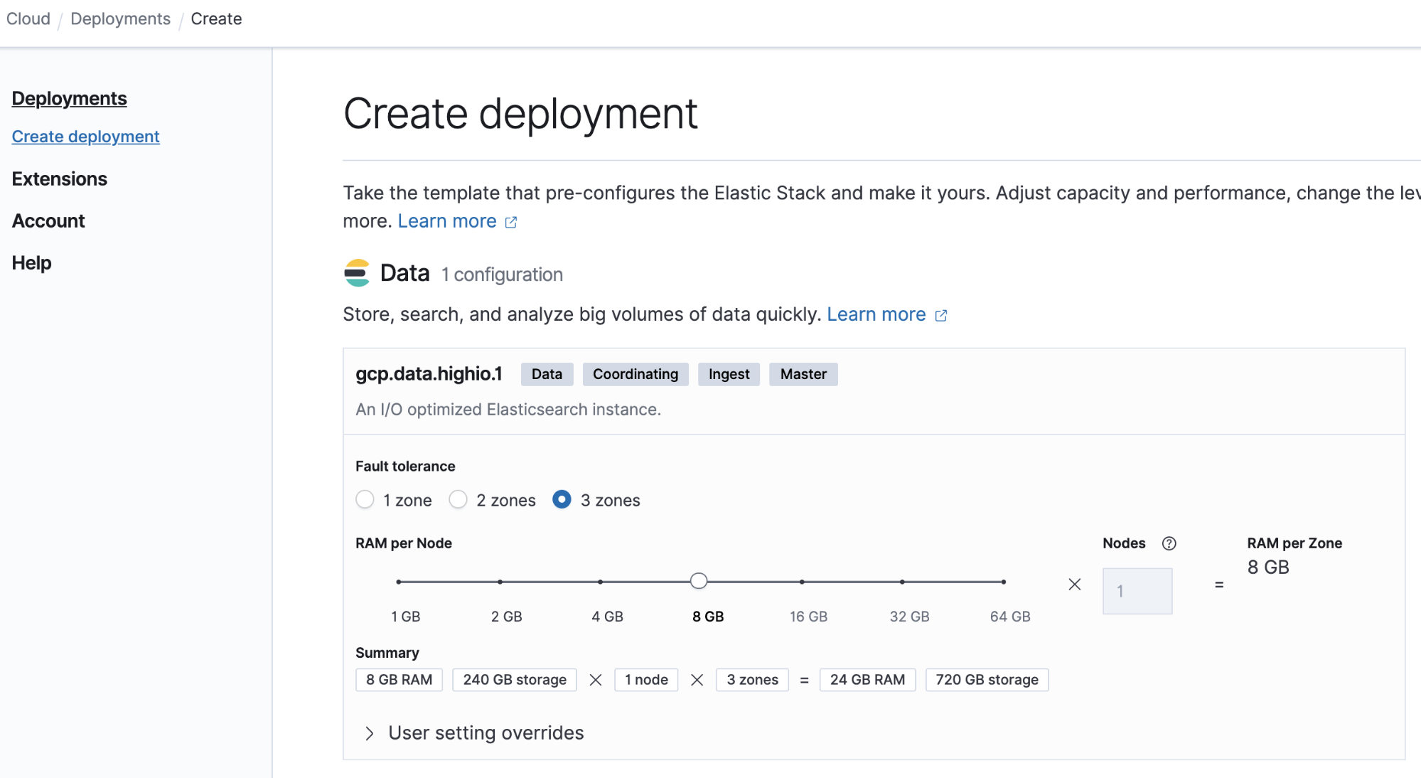
You can use 8GB memory per node for this small deployment. Let’s do the math:
- Total Data (GB) = 1GB x (9 x 30 days) x 2 = 540GB
- Total Storage (GB)= 540GB x (1+0.15+0.1) = 675GB
- Total Data Nodes = 675GB disk / 8GB RAM /30 ratio = 3 nodes
Let’s see how simple it is to build this deployment on Elastic Cloud:
Example: Sizing a large deployment
Your small deployment got successful and more partners want to use your Elasticsearch service, you may need resizing your cluster to much the new requirements.
Let’s do the math with the following inputs:
- You receive 100GB per day and we need to keep this data for 30 days in the hot zone and 12 months in the warm zone.
- We have 64GB of memory per node with 30GB allocated for heap and the remaining for OS cache.
- The typical memory:data ratio for the hot zone used is 1:30 and for the warm zone is 1:160.
If we receive 100GB per day and we have to keep this data for 30 days, this gives us:
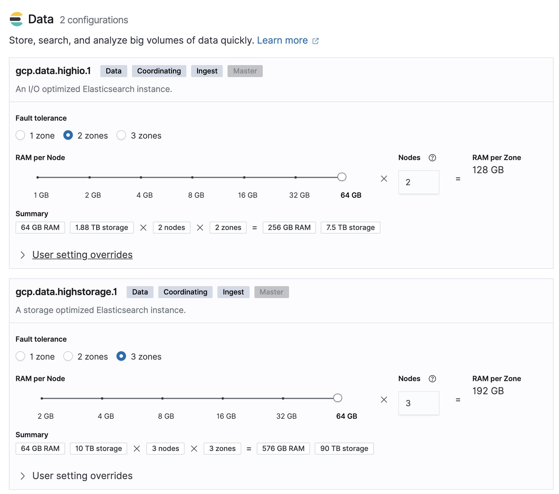
- Total Data (GB) in the hot zone = (100GB x 30 days * 2) = 6000GB
- Total Storage (GB) in the hot zone = 6000GB x (1+0.15+0.1) = 7500GB
- Total Data Nodes in the hot zone = ROUNDUP(7500 / 64 / 30) + 1 = 5 nodes
- Total Data (GB) in the warm zone = (100GB x 365 days * 2) = 73000GB
- Total Storage (GB) in the warm zone = 73000GB x (1+0.15+0.1) = 91250GB
- Total Data Nodes in the warm zone = ROUNDUP(91250 / 64 / 160) + 1 = 10 nodes
Let’s see how simple it is to build this deployment on Elastic Cloud:
Benchmarking
Now that we have our cluster(s) sized appropriately, we need to confirm that our math holds up in real world conditions. To be more confident before moving to production, we will want to do benchmark testing to confirm the expected performance, and the targeted SLA.
For this benchmark, we will use the same tool our Elasticsearch engineers use Rally. This tool is simple to deploy and execute, and completely configurable so you can test multiple scenarios. Learn more about how we use Rally at Elastic.
To simplify the result analysis, we will split the benchmark into two sections, indexing and search requests.
Indexing benchmark
For the indexing benchmarks we are trying to answers the following questions:
- What is the maximum indexing throughput for my clusters?
- What is the data volume that I can index per day?
- Is my cluster oversized or undersized ?
For the purpose of this benchmark we will use a 3 nodes cluster with the following configuration for each nodes:
- 8 vCPU
- Standard persistent disk (HDD)
- 32GB/16 heap
Indexing benchmark #1:
The data set used for this benchmark is Metricbeat data with the following specifications:
- 1,079,600 documents
- Data volume: 1.2GB
- AVG document size: 1.17 KB
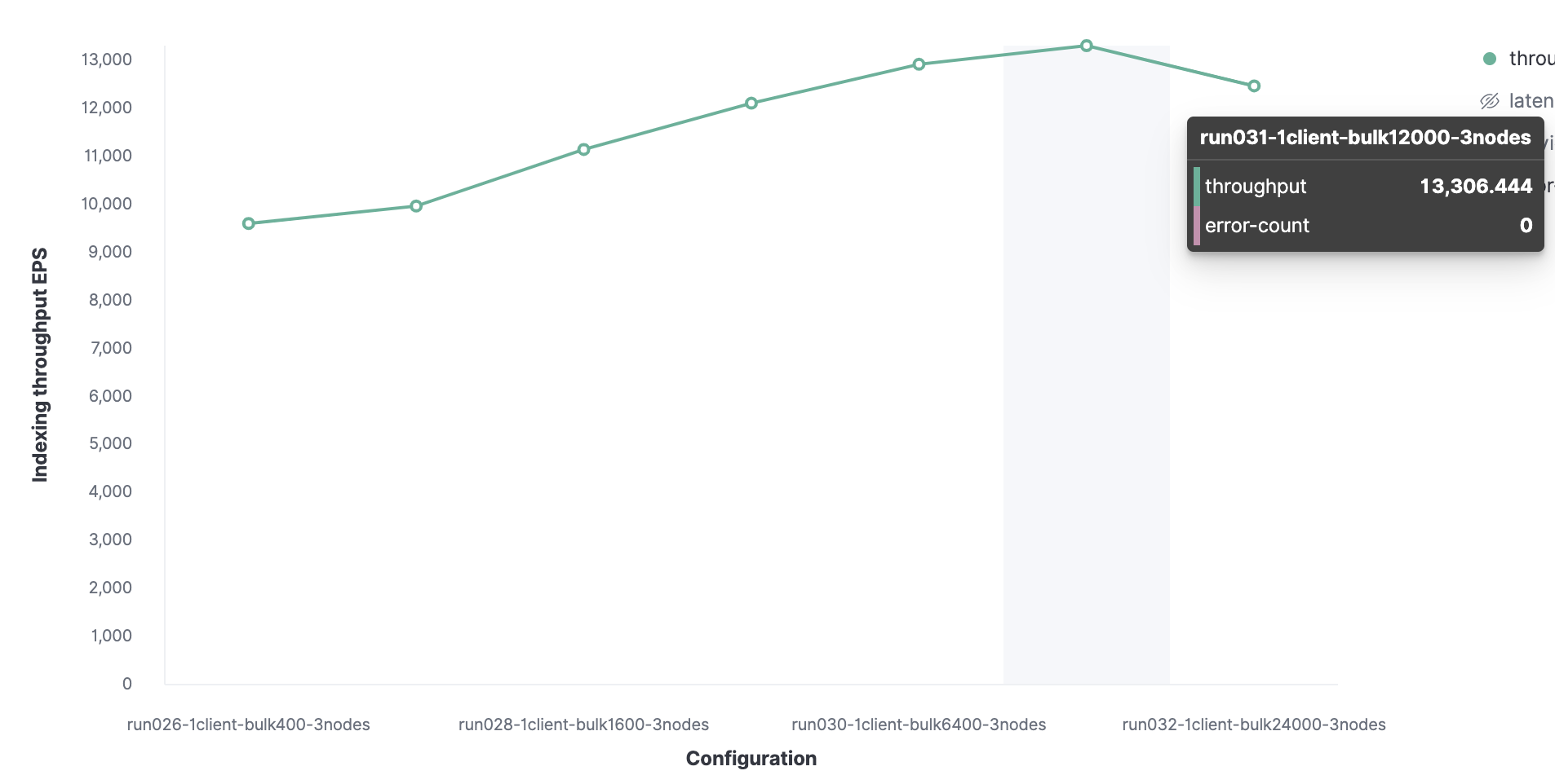
The indexing performance will depend also on the performance of the indexing layer, in our case Rally. We'll execute multiple benchmark runs to figure out the optimal bulk size and the optimal thread count in our case.
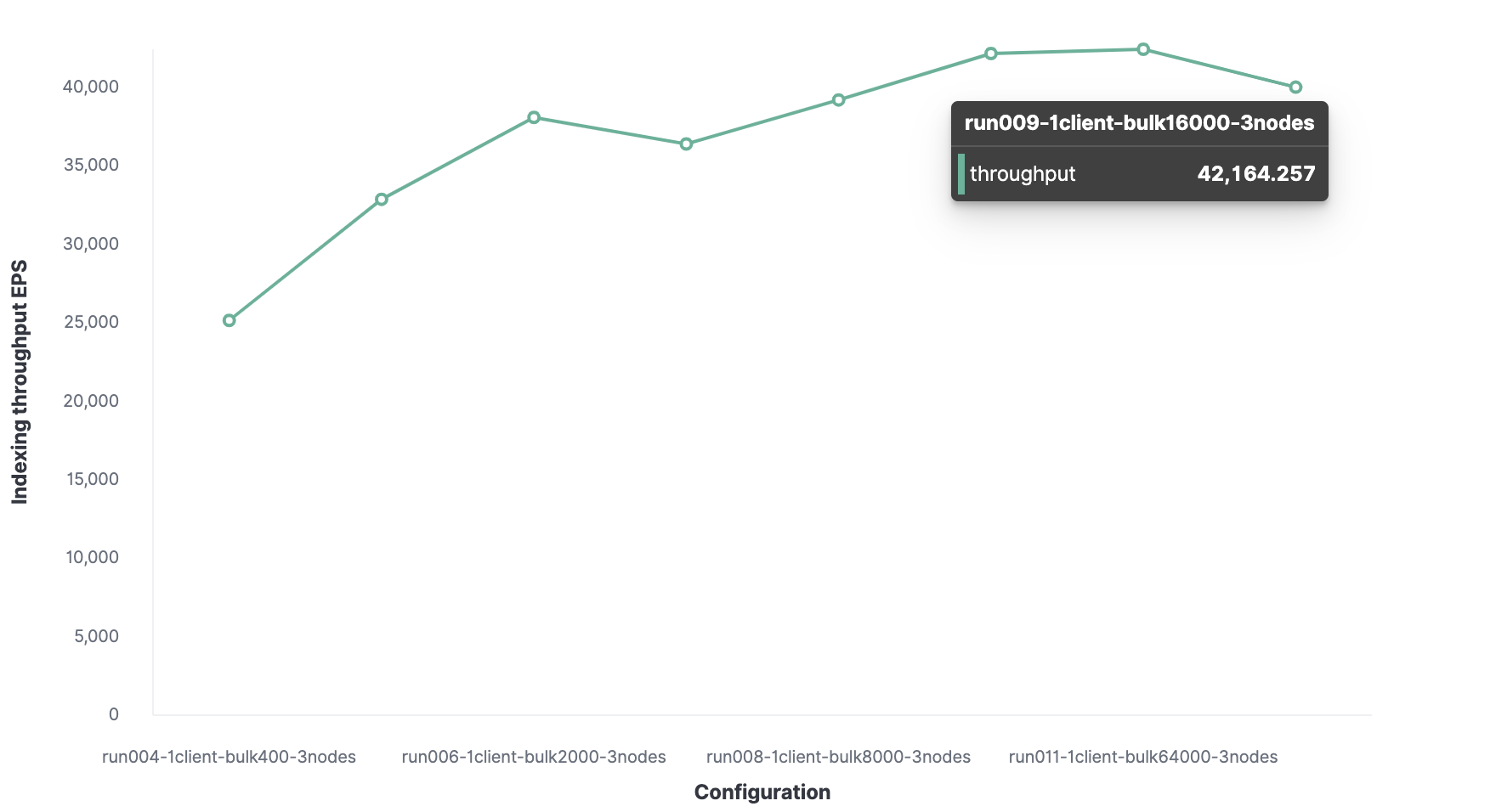
We’ll start with 1 Rally client to find the optimal batch size. Starting from 100, then increasing by double in subsequent runs, which shows that we have an optimal batch size of 12k (around 13.7 MB) and we can reach 13K events indexed per second.
Next, using a similar method, we find that the optimal number of clients is 16 allowing us to reach 62K events indexed per second.
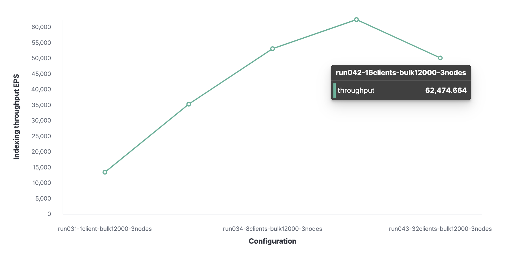
Our cluster can handle a maximum indexing throughput of 62K events per second. To go further we would need to add a new node.
I was curious to see how many indexing requests one node can handle, So I’ve executed the same track on a one node cluster and a two node cluster to see the difference.
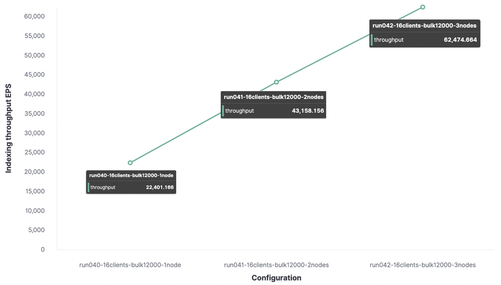
Conclusion: For my test environment, the maximum indexing throughput is...
- With 1 node and 1 shard we got 22K events per second.
- With 2 nodes and 2 shards we got 43k events per second.
- With 3 nodes and 3 shards we got 62k events per second.
Any additional indexing request will be put in the queue, and when the queue is full the node will send rejection responses.
Our dataset impacts the cluster performance, which is why it’s important to execute the tracks with your own data.
Indexing benchmark #2:
For the next step, I have executed the same tracks with the HTTP server log data using the following configuration:
- Volumes: 31.1GB
- Document: 247,249,096
- Avg document size: 0.8 KB
Optimal bulk size is 16K documents.
Yielding an optimal number of 32 clients.
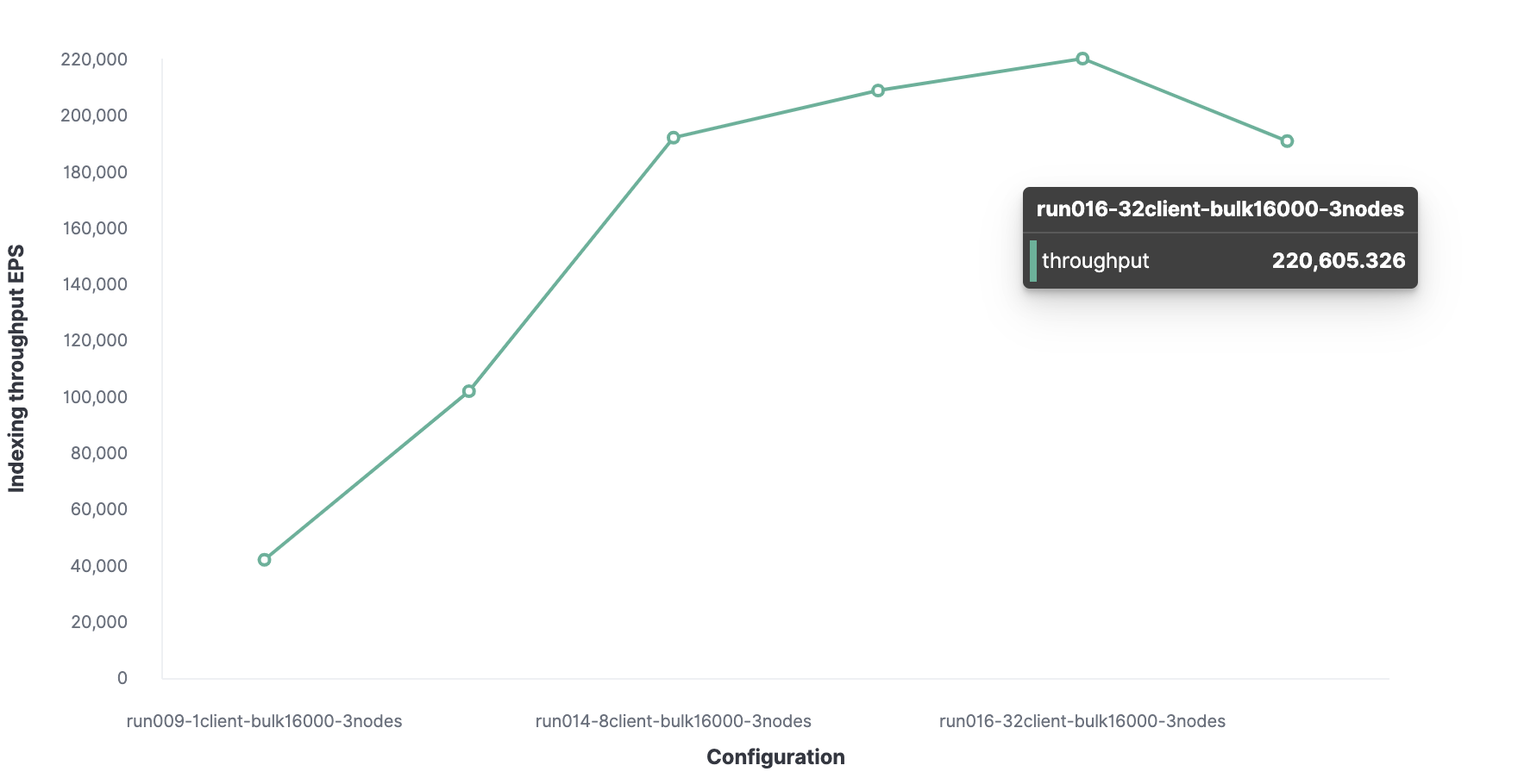
And the maximum indexing throughput for the http server log data is 220K events per second.
Search benchmark
To benchmark our search performance, we will consider using 20 clients with a targeted throughput of 1000 OPS.
For the search, we will execute three benchmarks:
1. Service time for queries
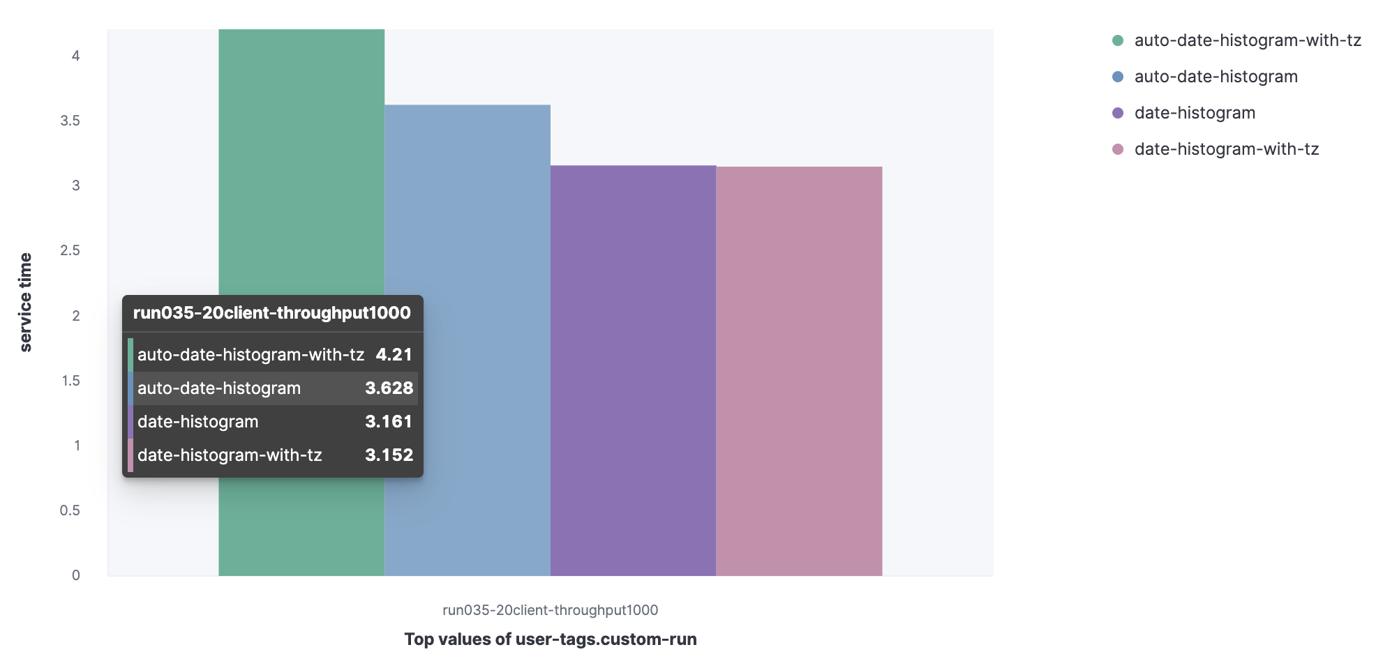
We will compare the service time (90 percentiles) for a set of queries.
Metricbeat data set
- auto-date-historgram
- auto-data-histogram-with-tz
- date-histogram
- Date-histogram-with-tz
We can observe that auto-data-histogram-with-tz query have the higher service time.
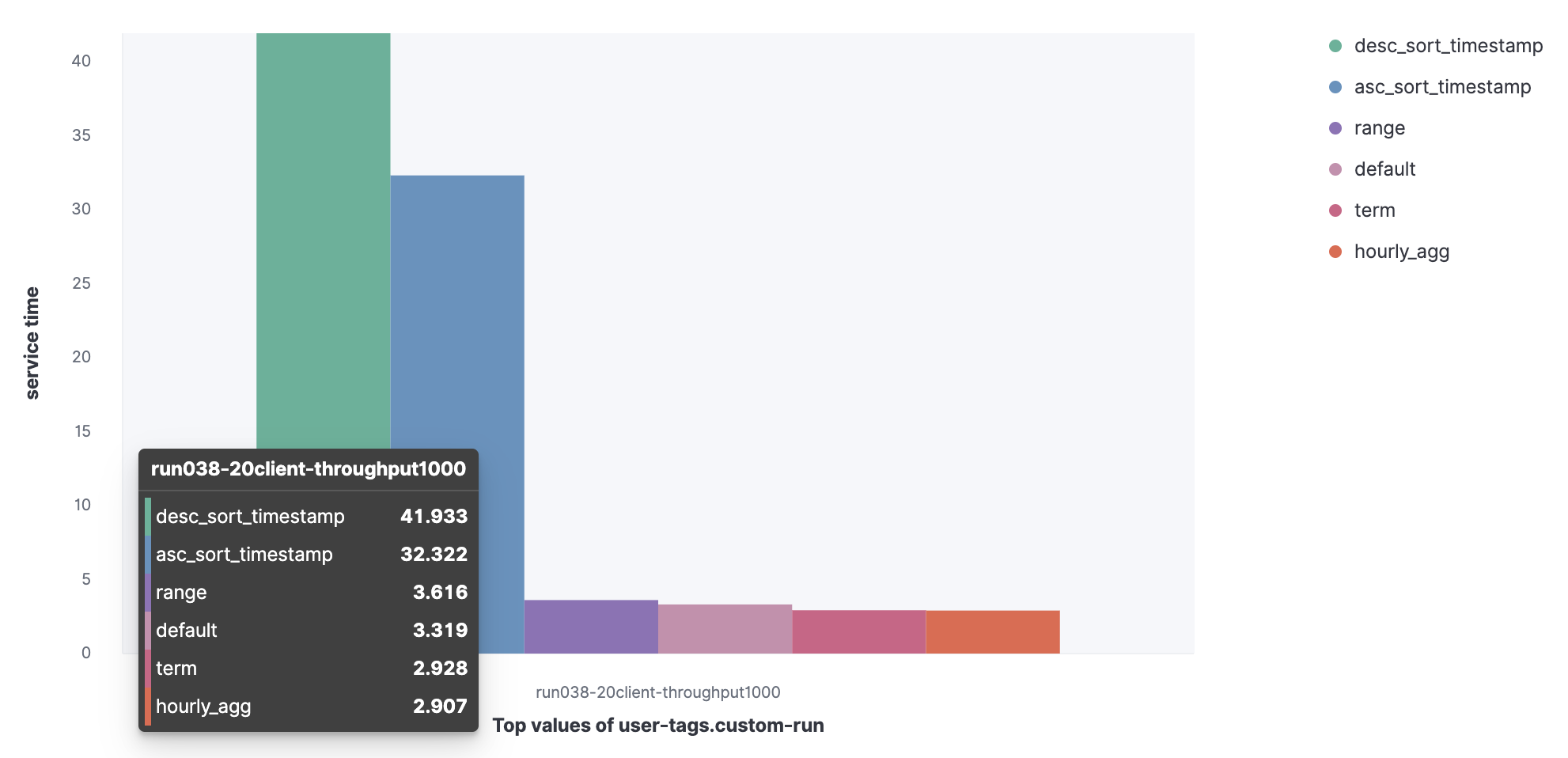
HTTP server log data set
- Default
- Term
- Range
- Hourly_agg
- Desc_sort_timestamp
- Asc_sort_timestamp
We can observe that desc_sort_timestamp and desc_sort_timestamp queries have the higher service time.
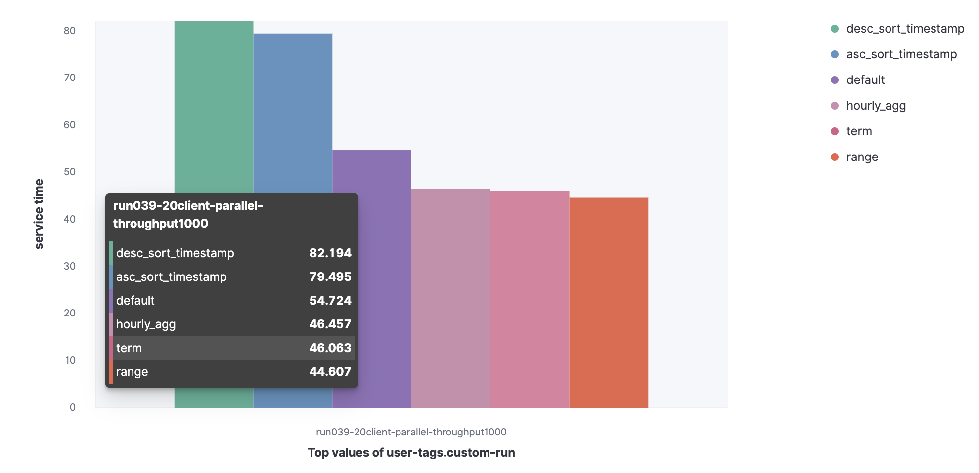
2. Service time for parallel queries
Let's see the 90 percentile service time increased if I execute the queries in parallel.
3. Index rate and service time with parallel indexing
We'll execute a parallel indexing task and the searches to see the indexing rate and the service time for our queries.
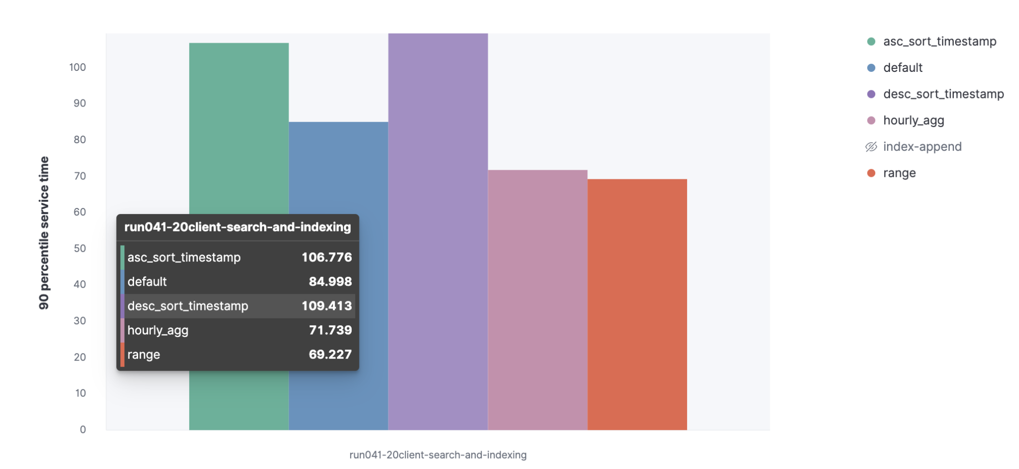
Let's see the 90 percentile service time for the queries increased when executing in parallel with indexing operations.
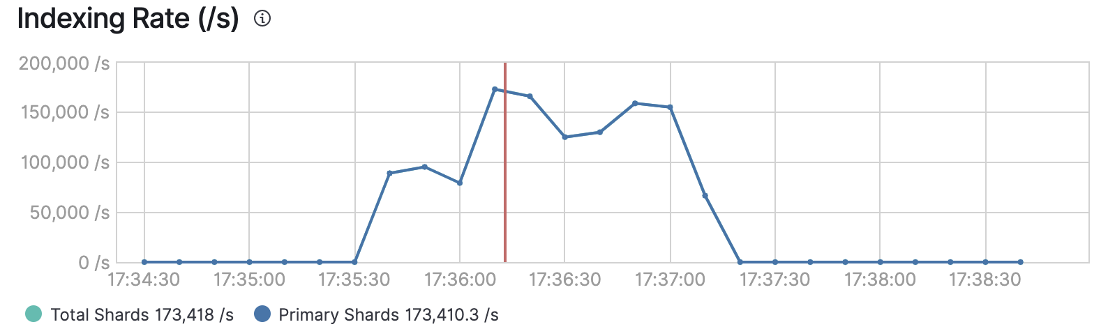
Reading our results
With 32 clients for indexing and 20 users for search we have:
- Indexing throughput 173K, less than 220K noted previously.
- Search throughput 1000 events per second.
Conclusion
The sizing exercise equips you with a set of methods to calculate the number of nodes that you need based on data volume. In order to best plan for the future performance of your cluster, you will also need to benchmark your infrastructure — something we've already taken care of in Elastic Cloud. Since the performance will depend also on your use case, we recommend using your data and your queries to be closest to the reality. More details about how to define a custom workload in the Rally documentation.
After the benchmark exercise, you should have a better understanding of your infrastructure performance and you can continue to fine tune Elasticsearch to improve your indexing speed. Additionally, learn how to use Rally to get your Elasticsearch right.