Identify slow queries in generative AI search experiences

A while ago, we introduced instrumentation inside Elasticsearch^®, allowing you to identify what it’s doing under the hood. By tracing in Elasticsearch, we get never-before-seen insights.

This blog walks you through the various APIs and transactions when we want to leverage the Elastic Learned Sparse EncodeR (ELSER) model for semantic search. This blog itself can be applied to any machine learning model running inside of Elasticsearch — you just need to alter the commands and searches accordingly. The instructions in this guide use our sparse encoder model (see docs page).

For the following tests, our data corpus is the OpenWebText, which provides roughly 40GB of pure text and roughly 8 million individual documents. This setup runs locally on a M1 Max Macbook with 32GB RAM. Any of the following transaction durations, query times, and other parameters are only applicable to this blog post. No inferences should be drawn to production usage or your installation.

The secret token (or API key) must be in the Elasticsearch keystore. The keystore tool should be available in <your elasticsearch install directory>/bin/elasticsearch-keystore using the following command elasticsearch-keystore add tracing.apm.secret_token or tracing.apm.api_key . After that, you need to restart your Elasticsearch. More information on tracing can be found in our tracing document.

Once this is activated, we can look in our APM view where we can see that Elasticsearch captures various API endpoints automatically. GET, POST, PUT, DELETE calls. With that sorted out, let us create the index:

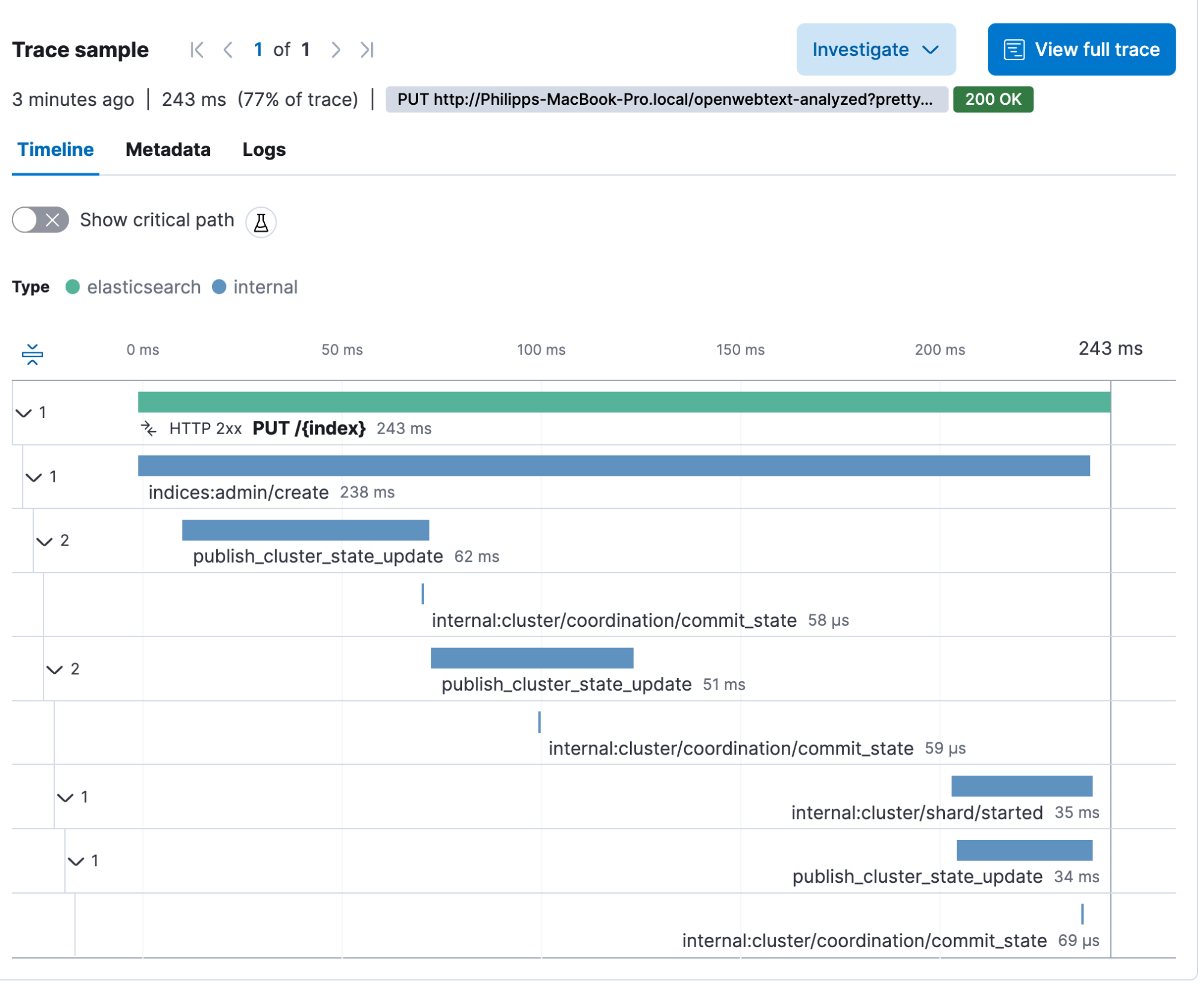
This should give us a single transaction called PUT /{index}. As we can see, a lot is happening when we create an index. We have the create call, we need to publish it to the cluster state and start the shard.

The next thing we need to do is create an ingest pipeline — we call it openwebtext. The pipeline name must be referenced in the index creation call above since we are setting it as the default pipeline. This ensures that every document sent against the index will automatically run through this pipeline if no other pipeline is specified in the request.

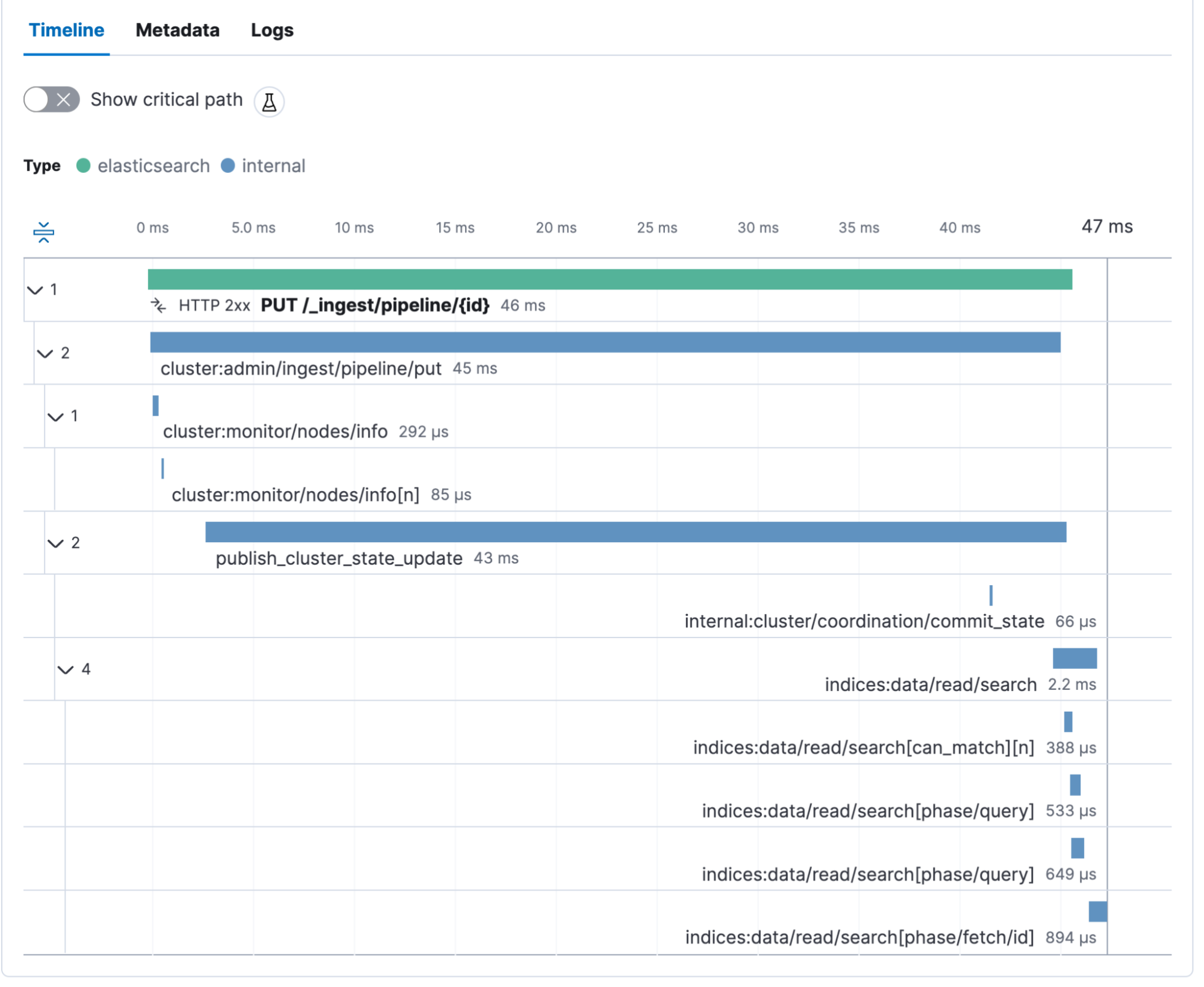
We get a PUT /_ingest/pipeline/{id} transaction. We see the cluster state update and some internal calls. With this, all the preparation is done, and we can start running the bulk indexing with the openwebtext data set.

Before we start the bulk ingest, we need to start the ELSER model. Go to Machine Learning, Trained Models, and click play. Here you can choose the number of allocations and threads.

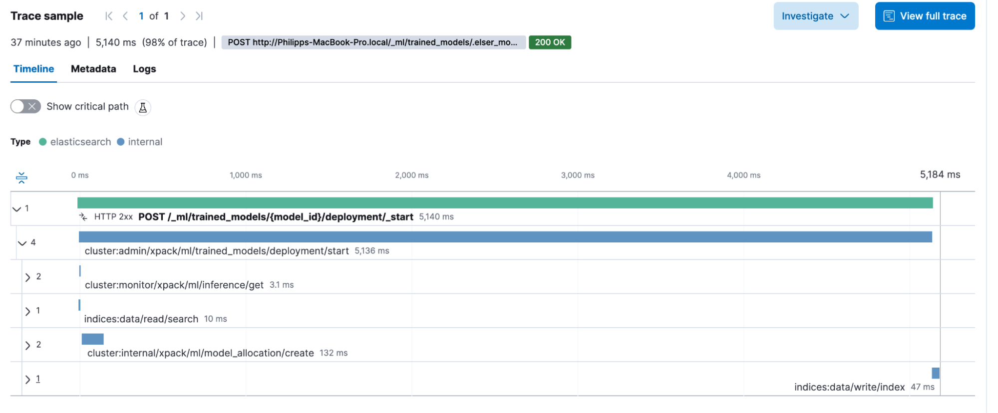
The model starts is captured as POST /_ml/trained_models/{model_id}/deployment/_start. It contains some internal calls and might be less interesting than the other transactions.

Now, we want to verify that everything works by running the following. Kibana Dev Tools have a cool little trick, you can use triple quotes, as in ””” at the start and the end of a text, to tell Kibana^® to treat it as a string and escape if necessary. No more manual escaping of JSONs or dealing with line breaks. Just drop in your text. This should return a text and a ml.tokens field showing all the tokens.

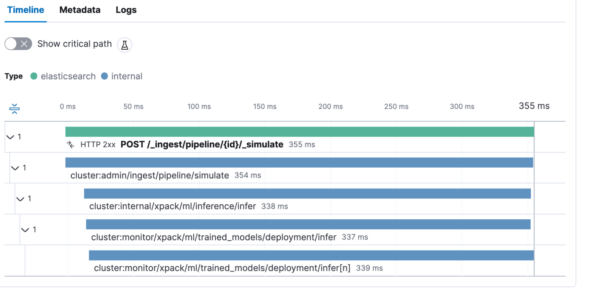
This call is also captured as a transaction POST _ingest/pipeline/{id}/_simulate. The interesting thing here is we see that the inference call took 338ms. This is the time needed by the model to create the vectors. 

The openwebtext data set has a single text file representing a single document in Elasticsearch. This rather hack-ish Python code reads all the files and sends them to Elasticsearch using the simple bulk helper. Note that you would not want to use this in production, as it is relatively slow since it runs in serialization. We have parallel bulk helpers allowing you to run multiple bulk requests at a time.

What is key information is that we are using a chunk_size of 25, meaning that we are sending 25 documents in a single bulk request. Let’s start this Python script. The Python helpers.bulk send a PUT /_bulk request. We can see the transaction. Every transaction represents a single bulk that contains 25 documents.

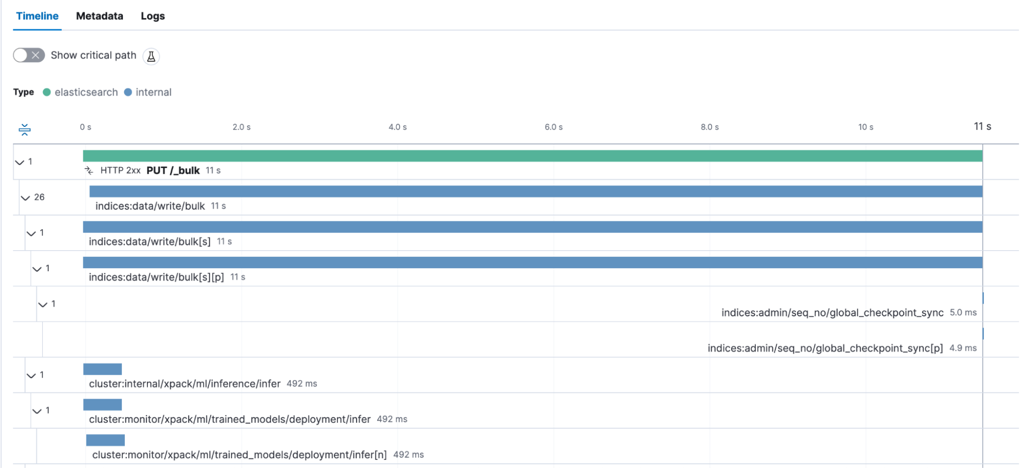
We see that these 25 documents took 11 seconds to be indexed. Every time the ingest pipeline calls the inference processor — and therefore, the machine learning model — we see how long this particular processor takes. In this case, it’s roughly 500 milliseconds — 25 docs, each ~500 ms processing ~= 12,5 seconds. Generally speaking, this is an interesting view, as a longer document might impose a higher tax because there is more to analyze than a shorter one. Overall, the entire bulk request duration also includes the answer back to the Python agent with the ok for the indexing. Now, we can create a dashboard and calculate the average bulk request duration. We’ll do a little trick inside Lens to calculate the average time per doc. I’ll show you how.

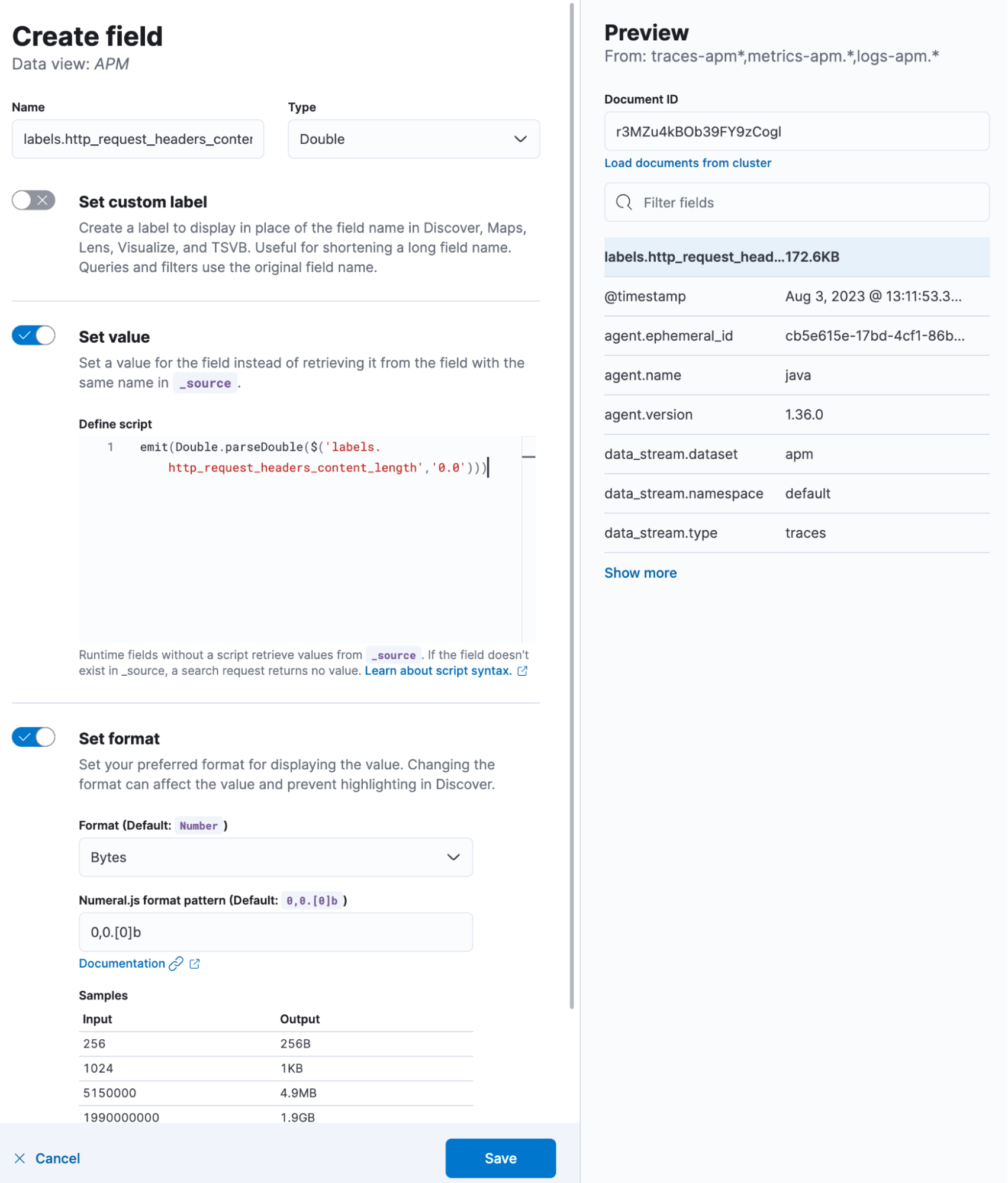
First, there is an interesting metadata captured inside the transaction — the field is called labels.http_request_headers_content_length. This field may be mapped as a keyword and therefore does not allow us to run mathematical operations like sum, average, and division. But thanks to runtime fields, we don’t mind that. We can just cast it as a Double. In Kibana, go to your data view that contains the traces-apm data stream and do the following as a value:

This emits the existing value as a Double if that field is non-existent and/or missing, and it will report as 0.0. Furthermore, set the Format to Bytes. This will make it automatically prettified! It should look like this:

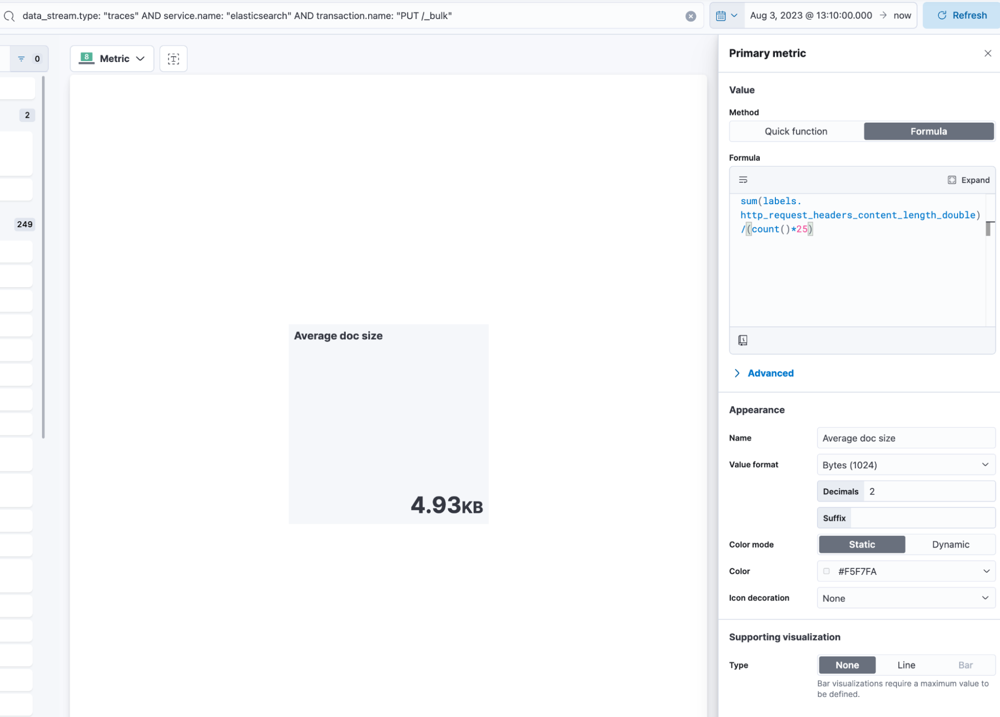
Create a new dashboard, and start with a new visualization. We want to select the metric visualization and use this KQL filter: data_stream.type: "traces" AND service.name: "elasticsearch" AND transaction.name: "PUT /_bulk". In data view, select the one that includes traces-apm, basically the same as where we added the field from above. Click on primary metric and formula:

Since we know that every bulk request contains 25 documents, we can just multiply the count of records (number of transactions) by 25 and divide the total sum of bytes to identify how large a single document was. But there are a few caveats — first, a bulk request includes an overhead. A bulk looks like this:

For every document you want to index, you get a second line in JSON that contributes to the overall size. More importantly, the second caveat is compression. When using any compression, we can only say “the documents in this bulk, where of size x” because the compression will work differently depending on the bulk content. When using a high compression value, we might end up with the same size when sending 500 documents compared to the 25 we do now. Nonetheless, it is an interesting metric.

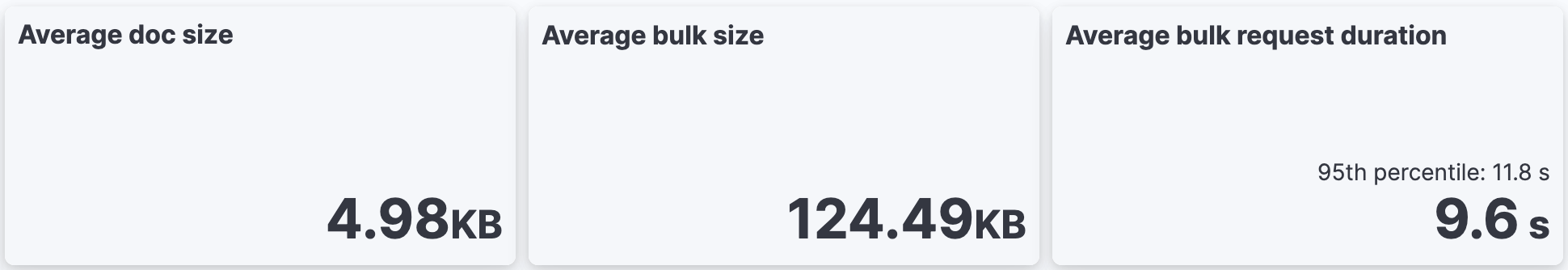
We can use the transaction.duration.us tip! Change the format in the Kibana Data View to Duration and select microseconds, ensuring it’s rendered nicely. Quickly, we can see that, on average, the bulk request is ~125kb in size, ~5kb per doc, and 9.6 seconds, with 95% of all bulk requests finishing below 11.8 seconds.

Now, we have indexed many documents and are finally ready to query it. Let’s do the following query:

I am asking the openwebtext data set on articles about feeding my cat medication. My REST client tells me that the entire search, from start to parsing the response, took: 94.4 milliseconds. The took statement inside the response is 91 milliseconds, meaning that the search took 91 milliseconds on Elasticsearch, excluding a few things. Let’s now look into our GET /{index}/_search transaction.

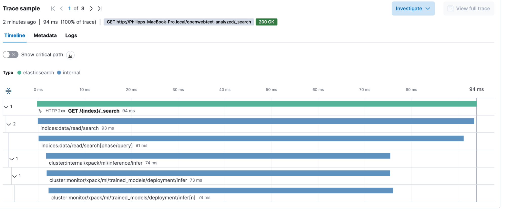
We can identify that the impact of the machine learning, basically creating the tokens on the fly, is 74 milliseconds out of the total request. Yes, this takes up roughly ¾ of the entire transaction duration. With this information, we can make informed decisions on how to scale the machine learning nodes to bring down the query time.

The release and timing of any features or functionality described in this post remain at Elastic's sole discretion. Any features or functionality not currently available may not be delivered on time or at all.