Explaining anomalies detected by Elastic machine learning


 Share on Twitter
Share on Twitter

 Share on LinkedIn
Share on LinkedIn

 Share on Facebook
Share on Facebook

 Share by Email
Share by Email

 Print this page
Print
Why is that anomalous? How come the anomaly score is not higher? Anomaly detection is a valuable machine learning feature used in Elastic Security and Observability. But, oh boy, those numbers can look confusing. If only someone could explain them in clear language. Or, even better, draw a picture.
In Elastic 8.6, we show extra details for anomaly records. These details allow looking behind the curtains of the anomaly scoring algorithm.
We have written about anomaly scoring and normalization in this blog before. The anomaly detection algorithm analyzes time series of data in an online fashion. It identifies trends and periodic patterns on different time scales, such as a day, a week, a month, or a year. Real-world data is usually a mix of trends and periodic patterns on different time scales. Moreover, what first looks like an anomaly can turn out to be an emerging recurring pattern.
The anomaly detection job comes up with hypotheses explaining the data. It weighs and mixes these hypotheses using the provided evidence. All hypotheses are probability distributions. Hence, we can give a confidence interval on how "normal" the observations are. Observations that fall out of this confidence interval are anomalous.
Anomaly score impact factors
Now, you probably think: Well, this theory is straightforward. But once we see some unexpected behavior, how do we quantify how out of the ordinary it is?
Three factors can constitute the initial anomaly score we give to the records:
- Single bucket impact
- Multi bucket impact
- Anomaly characteristics impact
To remind you, anomaly detection jobs split the time series data into time buckets. The data within a bucket is aggregated using functions. Anomaly detection is happening on the bucket values. Read this blog post to learn more about buckets and why choosing the right bucket span is critical.
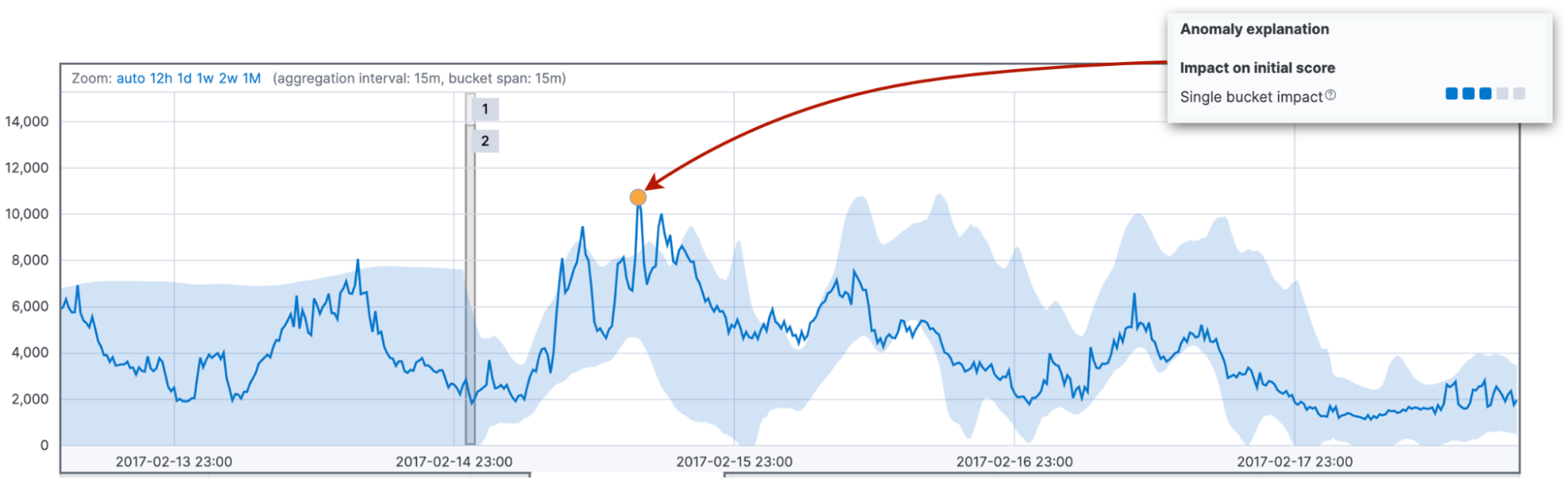
First, we look at the probability of the actual value in the bucket, given the hypotheses mixture. This probability depends on how many similar values we have seen in the past. Often, it relates to the difference between the actual value and the typical value. The typical value is the median value of the probability distribution for the bucket. This probability leads to the single bucket impact. It usually dominates the initial anomaly score of a short spike or dip.
Second, we look at the probabilities of observing the values in the current bucket values together with the preceding 11 buckets. The accumulated differences between the actual and typical values result in the multi bucket impact on the initial anomaly score of the current bucket.
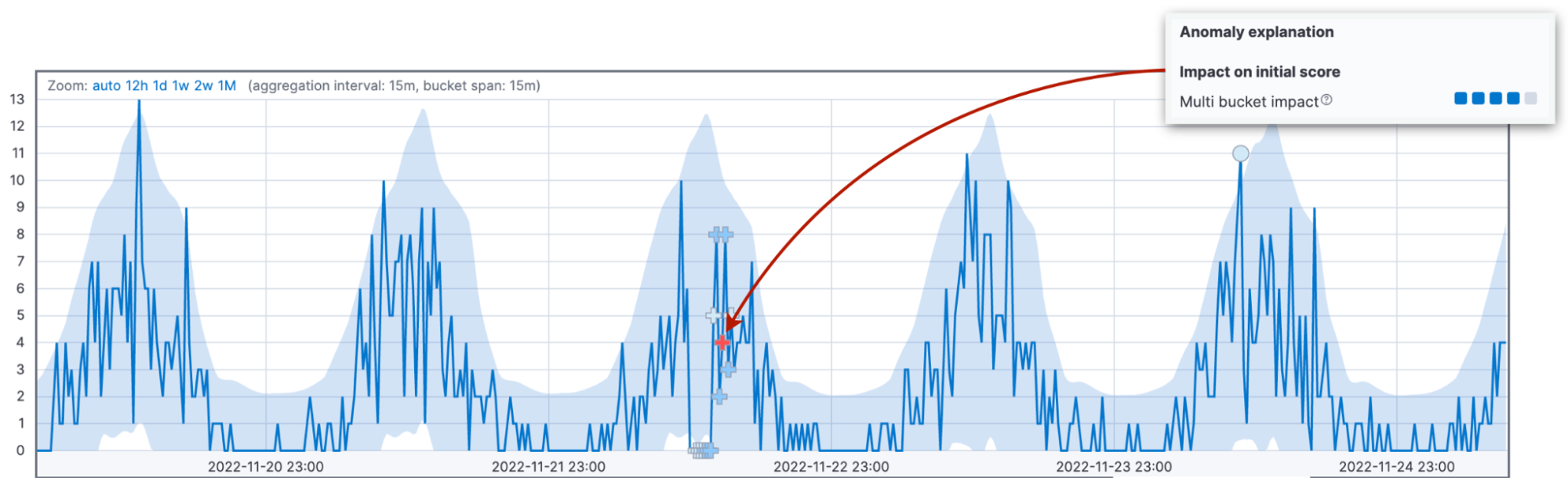
Let's dwell on this idea since the multi bucket impact is the second most common cause of confusion about anomaly scores. We look at the combined deviations in 12 buckets and assign the impact to the current bucket. High multi bucket impact indicates unusual behavior in the interval preceding the current bucket. Never mind that the current bucket value may be back within the 95% confidence interval.
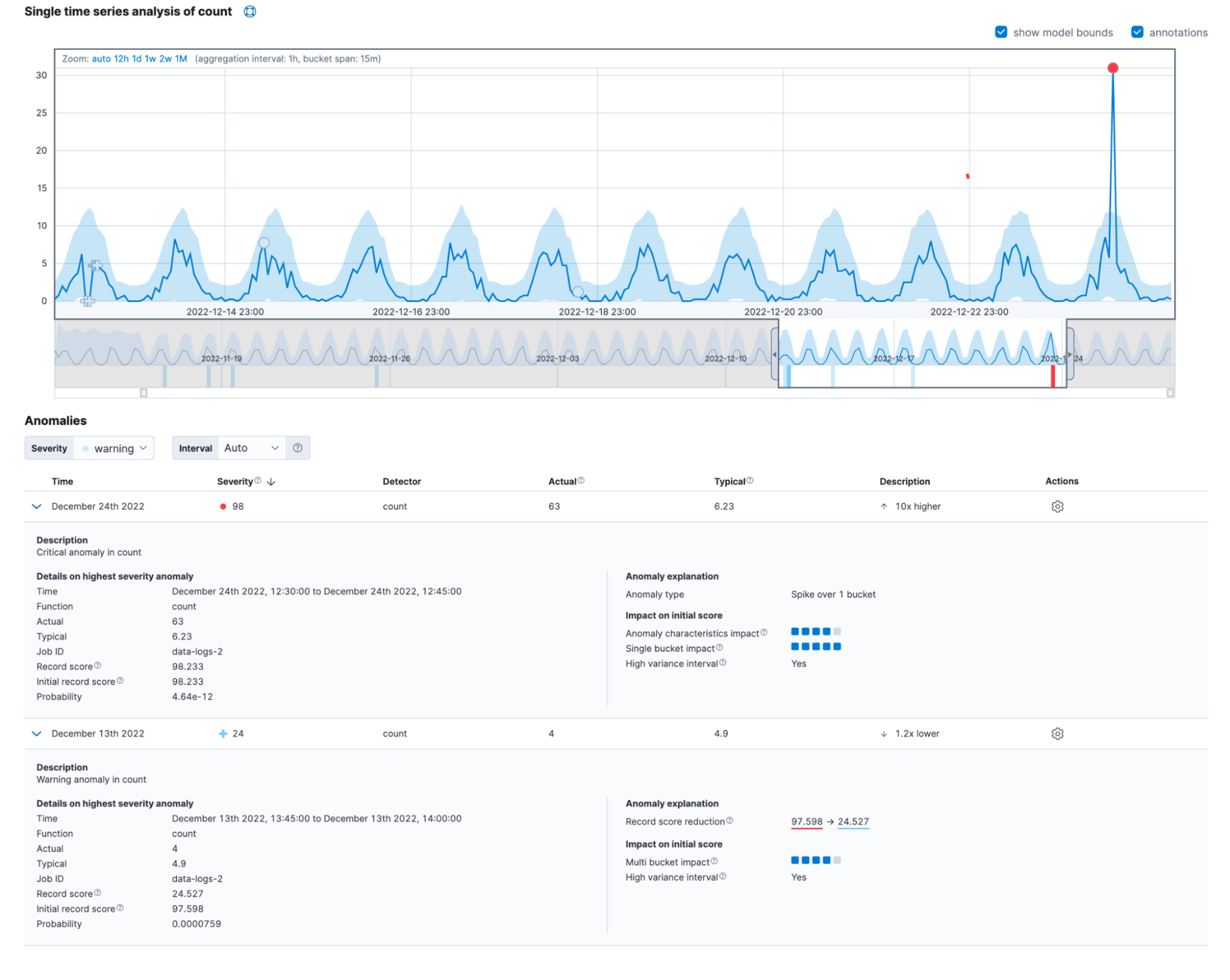
To highlight this difference, we even use different markers for anomalies with high multi bucket impact. If you look closely at the multi bucket anomaly in the figure above, you can see that the anomaly is marked with a cross sign "+" instead of a circle.
Finally, we consider the impact of the anomaly characteristics, such as the length and the size. Here we take into account the total duration of the anomaly until now, not a fixed interval as above. It can be one bucket or thirty. Comparing the length and size of the anomaly to the historical averages allows for adapting to the customer domain and patterns in data.
Moreover, the default behavior of the algorithm is to score longer anomalies higher than short-lived spikes. In practice, short anomalies often turn out to be glitches in data, while long anomalies are something you need to react to.
Why do we need both factors with fixed and variable intervals? Combining them leads to more reliable detection of abnormal behavior over various domains.
Record score reduction
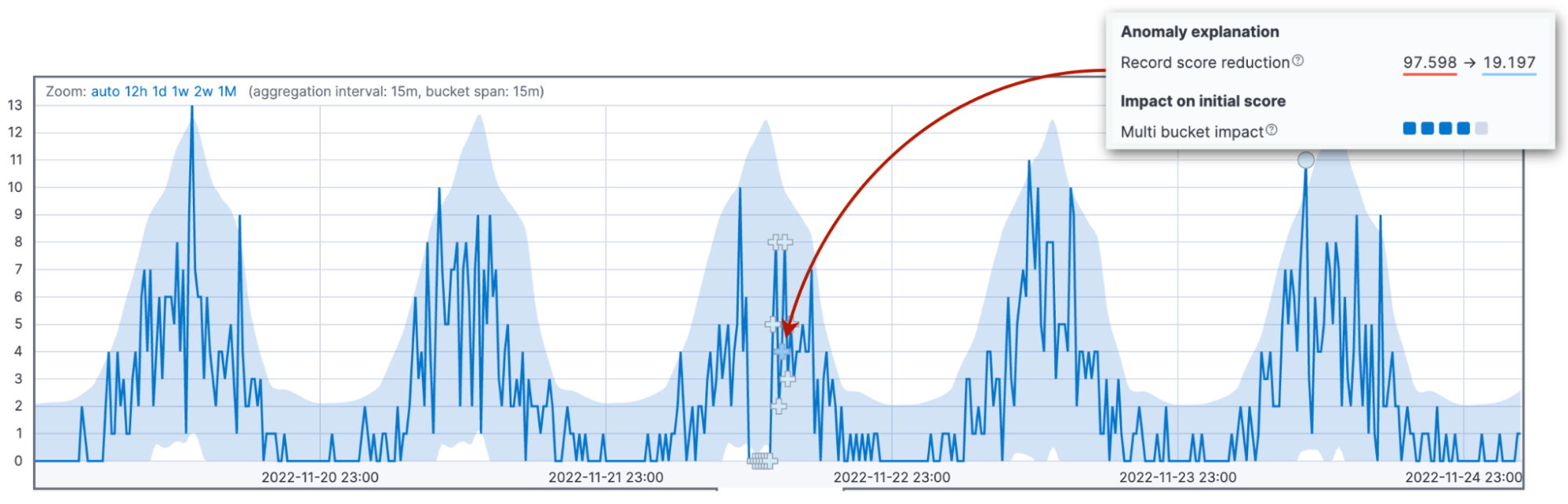
Now, it's time to talk about the most common source of scoring confusion: score renormalization. Anomaly scores are normalized into the range between 0 and 100. The values close to 100 signify the biggest anomalies the job has seen to date. This means that when we see an anomaly bigger than ever before, we need to reduce the scores of previous anomalies.
The three factors described above impact the value of the initial anomaly score. The initial score is important because the operator gets alerted based on this value. As new data arrives, the anomaly detection algorithm adjusts the anomaly scores of the past records. The configuration parameter renormalization_window_days specifies the time interval for this adjustment. Hence, if you are wondering why an extreme anomaly shows a low anomaly score, it may be because the job has seen even more significant anomalies later.
The Single Metric Viewer in Kibana version 8.6 highlights this change.
Other factors for score reduction
Two more factors may lead to a reduction of the initial score: high variance interval and incomplete bucket.
Anomaly detection is less reliable if the current bucket is part of a seasonal pattern with high variability in data. For example, you may have server maintenance jobs running every night at midnight. These jobs can lead to high variability in the latency of request processing.
Also, it is more reliable if the current bucket has received a similar number of observations as historically expected.
Putting it all together
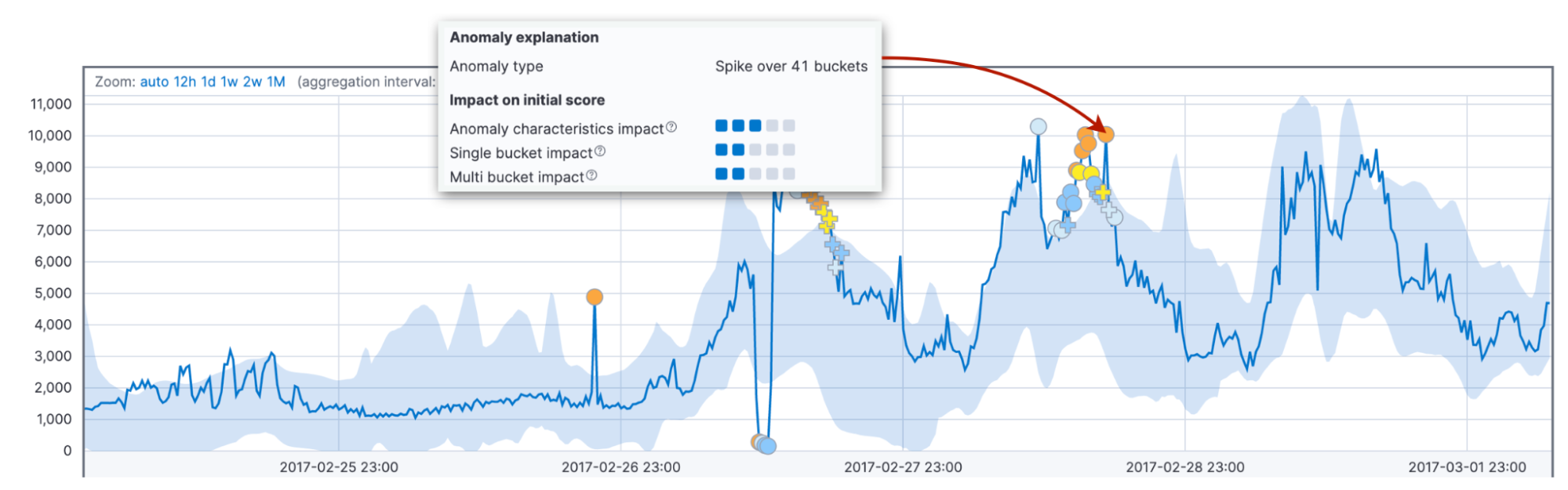
Often, real-world anomalies exhibit the impacts of several factors. Altogether, the new detailed view of the single metric viewer can look as follows.
You can also find this information in the anomaly_score_explanation field of the get record API.
Conclusion
You should try the latest version of Elasticsearch Service on Elastic Cloud and look at the new detailed view of anomaly records. Start your free Elastic Cloud trial today to access the platform. Happy experimenting!
Share
- Share on Twitter
Share on Twitter
- Share on LinkedIn
Share on LinkedIn
- Share on Facebook
Share on Facebook
- Share by Email
Share by Email
- Print this page
Print