Benchmarking binary classification results in Elastic machine learning
Binary classification aims to separate elements of a given dataset into two groups on the basis of some learned classification rule. It has extensive applications from security analytics, fraud detection, malware identification, and much more. Being a supervised machine learning method, binary classification relies on the presence of labeled training data that can be used as examples from which a model can learn what separates the classes. For example, to create a malware identification system, a binary classification model that separates malicious from benign binaries would need to first see proper examples from each class.
In the past few months we’ve released many new features in machine learning, all centered around supervised machine learning. Based on our research, Elastic’s binary classification implementation outperforms other known binary classification models when compared using a suite of open datasets.
Supervised vs. unsupervised learning
What is binary classification? To get started, let’s first discuss where it fits in in the machine learning landscape. Binary classification is a type of supervised machine learning problem — a task in which we train models that learn how to map inputs to outputs on labeled data — we’ll see an example of this below. This differs from unsupervised learning (anomaly detection, categorization, and outlier detection) in that in unsupervised learning our goal is to model the underlying structure of and existing patterns in data.
Unsupervised
For example, in time series anomaly detection, we have no a priori knowledge about which periods contain anomalous behavior, all we have are the individual data points that make up the time series. In the below figure, we’ve modeled the underlying structure of, and patterns in, the time series and determined what its “normal” bounds are. Any deviations from this normal range are anomalous and marked as such.

Supervised
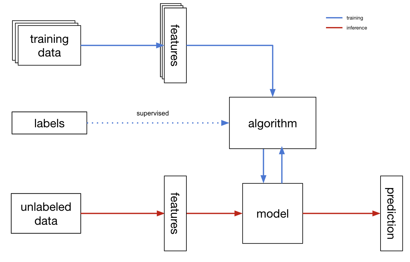
Contrast this example with a supervised learning task. In supervised learning, we train a machine learning model on training data which contains examples of the correct associations between inputs and outputs.
Let’s imagine we’re part of a security analytics team responsible for tracking down malicious connections to our company’s servers. Each day we go through hundreds of connections marking each one as benign or malicious. As our company grows and the number of connections increases to a point where we cannot feasibly manually track each connection, we need to scale this process. How might we go about this? We could take the unsupervised approach by modeling typical connections and then marking any connections that deviate from the “norm” as malicious. However this would be ignoring all of our previous manual tagging work! We have a huge set of labeled data that we collated while we were still manually tracking connections; we can use this to train a supervised classification model.
Binary classification
Back to binary classification — what is it? Binary classification is the task of categorizing data points into one of two groups. Typical uses for binary classification include fraud detection, security analytics, quality control, or information retrieval. Our security analytics example above is a prime use case for binary classification, so let’s dig a bit deeper into how we’d set up this problem.
Each connection has a number of different attributes which uniquely describe it, we call these features. For example, a connection might appear as follows:
When our hypothetical company was still young, our security analysts pored through our incoming connections and manually enriched each one with a tag that indicates whether the connection was benign or malicious. This provides us with a great training data set.
Now that we have our training data, how can we train a binary classification model? There are many different types of models, including decision trees, random forests, support vector machines, and neural networks; for this example, let’s look at a simple decision tree.
Decision trees are quite simple to understand and also serve as the foundation of our binary classification implementation, which is based off of XGBoost — a type of gradient boosted decision tree. You can think of a decision tree as an upside-down tree where the leaves are classes and each branch of the tree is a different attribute. Viewed in this way, we can think of a decision tree as a learned set of rules or series of questions that you can ask of each individual data point to determine its class.
Let’s follow our connection through an example tree to determine its status:
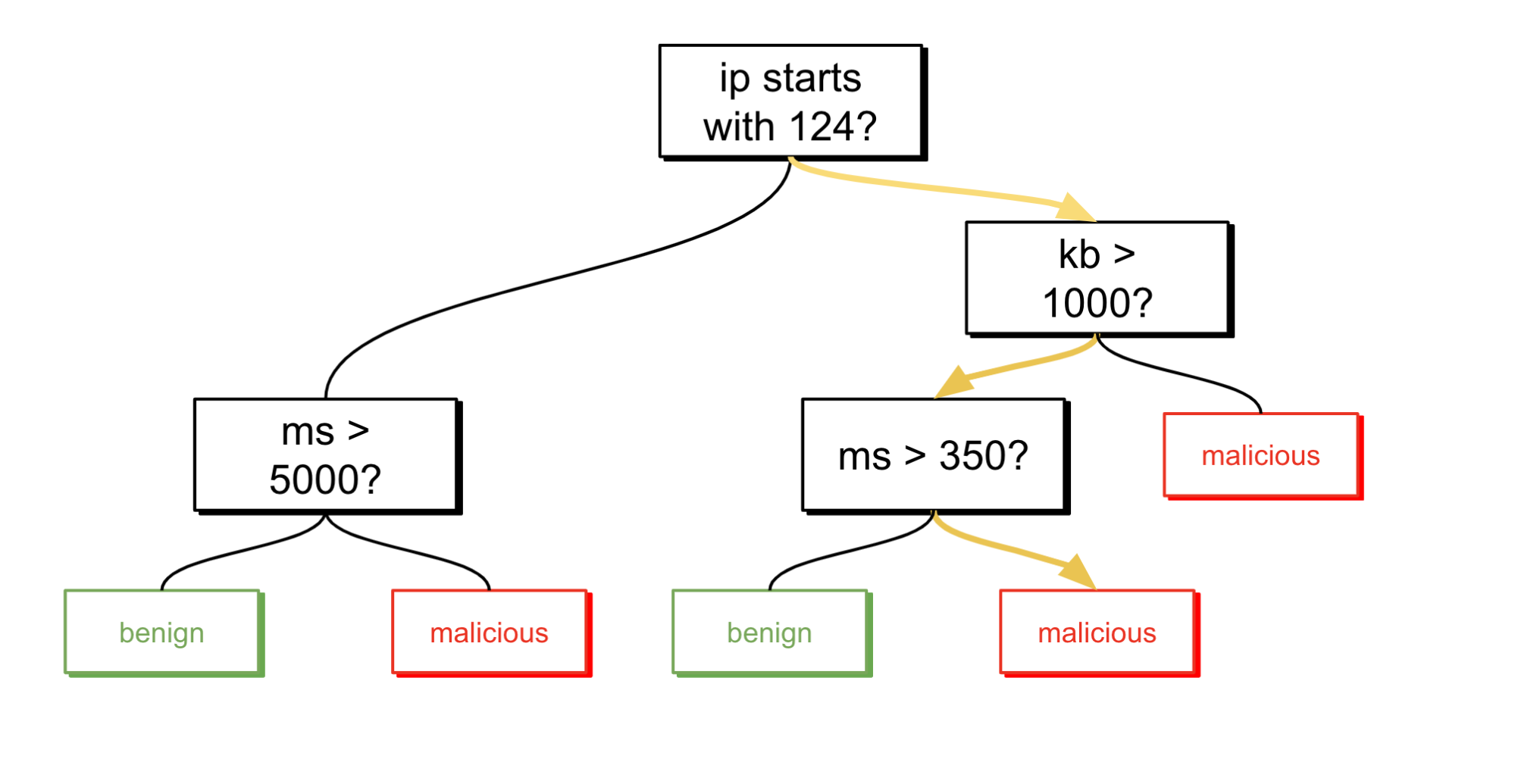
Uh oh! Looks like we have a bad one.
The algorithm that we use to train classification models is an ensemble method that combines gradient boosting with decision trees. Gradient boosting is a technique that trains many weak learners (in our case, decision trees) sequentially until each subsequent improvement on training is minimal.
Elastic classification excels in comparison
Experimental setup
While developing binary classification, we continuously referenced datasets and runs from OpenML, which is best described by their mission statement:
OpenML is an inclusive movement to build an open, organized, online ecosystem for machine learning. We build open source tools to discover (and share) open data from any domain, easily draw them into your favorite machine learning environments, quickly build models alongside (and together with) thousands of other data scientists, analyze your results against the state of the art, and even get automatic advice on how to build better models. Stand on the shoulders of giants and make the world a better place.
OpenML is an invaluable tool and has provided us with many, many high quality results against which to benchmark.
For this benchmarking, we chose to compare our results against other binary classification algorithms’ runs on the OpenML Curated Classification Suite 2018. This suite contains 72 datasets, 35 of which have binary targets, and 31 of which were used in this benchmark. We omitted 4 datasets that had greater than 100 features because of relatively long runtimes required to analyze them.
For each dataset, we chose the top 10,000 runs based on predictive accuracy, a measure that represents the number of true results among the total number of cases examined.
Comparison of binary classification algorithms’ performance
First, we look at Elastic’s out-of-the-box performance against all algorithms used by OpenML runs on these benchmark datasets. A total of 318,520 runs are compared in the box and whisker plots, covering a variety of different algorithms utilizing different parameter values across different implementations. To generate Elastic’s figures, we averaged the predictive accuracy of five runs of our binary classification analysis. Also, when running classification with Elastic, no parameters are required to be set by the user — the analysis process automatically sets parameters by default by estimating them via cross validation-error. Of course, it is possible to override these parameters through the classification configuration. This is markedly different from the other algorithms which requires user supplied values for the parameters.
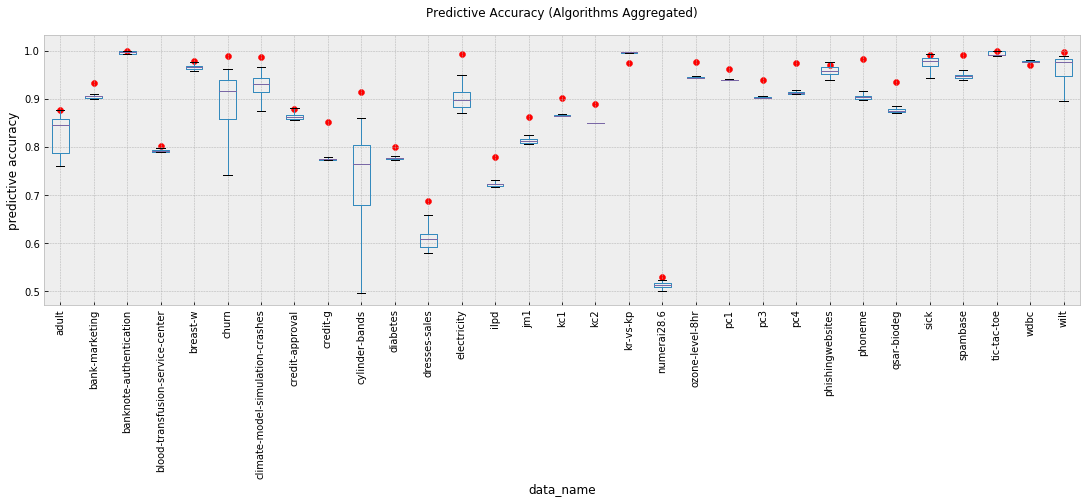
Elastic’s performance is indicated by the red circles. On average, we see a 5.1% improvement in mean accuracy when using Elastic’s binary classification. Elastic’s best run exceeded the best OpenML run in 26 of the 31 datasets, matched the best OpenML run in 2 of the 5 remaining datasets, and for 2 of the remaining 3 datasets, Elastic’s accuracy differed from the best OpenML result by less than one half of one percentage point.
For each of the 31 datasets, we ran 5 Elastic binary classification analyses, totaling 155 jobs. Running the complete benchmark took roughly 6 hours on a personal laptop, meaning average runtime was just over 2 minutes per analysis.
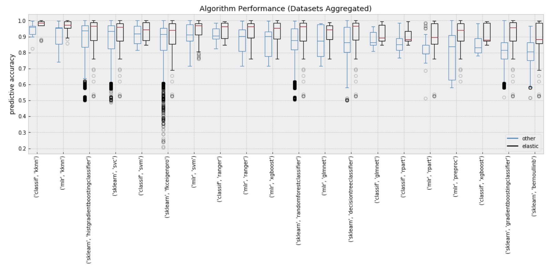
This second figure compares Elastic’s range of performance against each algorithm and implementation.
The implementations compared here contain:
- mlr — R package for Machine Learning
- sklearn — Python package for machine learning
- classif — Indicates that the method used was not part of a library but directly from the package itself. The packages include:
Conclusion
Binary classification is just one of our brand new features that offer supervised learning in the Elastic Stack! You can try it out today with a free 14-day trial. We are excited to offer methods that are competitive with state-of-the-art binary classification algorithms and would love to hear more about how you are making classification work for your use cases. Enjoy!
For more information about data frames, transforms, and supervised learning, check out this material: