Skip the mapping explosion: ES|QL queries schemaless JSON keys without dynamic mapping

ES|QL now reads flattened fields. FIELD_EXTRACT pulls any key out of a schemaless JSON object so you can filter, group, sort and join on keys you never mapped. The planner pushes those predicates into the columnar store rather than parsing the whole blob per row, which means dynamic JSON keys from OTel attributes, log labels, user metadata or whatever else you didn't want to map individually are queryable without causing a mapping explosion.

Why dynamic mapping breaks down with schemaless data

Elasticsearch wants a schema. Every field you index has a mapping that defines its type, its analyzer (for text), and how it is stored. That schema makes storage compression efficient, with fast search and cheap aggregation. It becomes a liability the moment your data stops looking like a database table.

Consider the shapes that show up in real systems:

• Log events where every service adds its own attributes. One emits labels.region, another labels.k8s.pod, and another labels.tenant_id.

• OpenTelemetry resource attributes, where the set of keys is defined by whatever agent happened to send the span.

• User-supplied metadata bags, feature flags, or tagging systems, where the keys are open-ended by design.

If you map each key as its own field, the mapping grows unbounded. This is the classic "mapping explosion." Thousands of dynamically created fields inflate the cluster state, slowing down every mapping update and eventually hitting the field limit. Each field also carries overhead in the index. You pay a structural cost for keys you didn’t plan for and may query only once.

The naive escape hatch is to store the whole object as a string and give up on querying its contents. That trades one problem for another: you keep the data but lose the ability to filter or group by anything inside it.

The flattened field type is the better path. You can index an entire JSON object under a single mapped field, keeping the keys queryable with almost none of the mapping-explosion cost. 

This post covers how a flattened field stores the data on a disk and how ES|QL reads it back.

How flattened fields index dynamic JSON keys under one mapping

Map one field as flattened:

PUT logs
{
 "mappings": {
"properties": {
"labels": { "type": "flattened" }
   }
 }
}

Then write arbitrary nested JSON into it:

POST logs/_doc
{
 "labels": {
   "region": "us-east-1",
   "k8s": { "pod": "web-7f9", "node": "ip-10-0-0-3" },
   "retries": 4
 }
}

There is exactly one field in the mapping, labels, no matter how many keys appear across your documents. The cluster state doesn’t grow when a new key shows up. The subkeys remain individually searchable. You can reference labels.region or labels.k8s.pod in queries, even though neither was ever declared.

The catch and central tradeoff is that every leaf value is a keyword. The number 4 above is indexed as the string "4". There is no numeric typing, no date parsing, and no range math on dynamic keys. Flattened fields exchange per-field richness for schema flexibility. That fact explains almost every design decision that follows.

How Elasticsearch stores flattened field JSON keys on disk

There are two types of queries on flattened fields: an unkeyed query on the root flattened field, and a keyed query on a specific subfield. Following the previous example, a query of the form labels: "us-east-1" matches a value under any key, while the querylabels.region: "us-east-1" matches a value under the specific regionkey.

To support these two distinct query formats, the flattened mapper writes each leaf value into two distinct Lucene fields.

Take this document:

{ "labels": { "region": "us-east-1", "k8s": { "pod": "web-7f9" } } }

The mapper produces:

• A root field under labels, holding the bare values:

us-east-1
web-7f9

• A keyed field under labels._keyed, holding the flattened key concatenated with its value:

region\0us-east-1
k8s.pod\0web-7f9

In the keyed field, nested objects are dot-flattened into a single key (k8s.pod), and the key is joined to its value with a reserved NULL byte (\0) as the separator. Keys that contain a NULL byte are rejected at parse time, so the separator is always unambiguous. To find the value, you split on the first NULL.

These two fields make both query shapes work:

• labels: "us-east-1" matches a value under any key, so it searches the root field.

• labels.region: "us-east-1" matches a value under a specific key. It rewrites the query to the term region\0us-east-1 and searches the keyed field.

Query restrictions on flattened field subkeys

Because every key's terms live in one sorted list, the keyed field cannot answer every query shape a plain keyword field can. Three restrictions follow:

1. No fuzzy, regexp, or wildcard on a specific subkey. Nothing about the layout makes them impossible,  but the pattern would have to be combined with the key prefix so it can’t walk past the key boundary. The mapper doesn’t do that at this writing.

2. Any range query on a subkey needs at least one bound. Elasticsearch already has a query for "this field has some value here, whatever it is": the exists query. On a flattened subkey it runs as a prefix query on key\0, which sweeps every term belonging to that key. A range with neither bound would sweep exactly the same terms. Rather than support two spellings of one scan, the mapper rejects the boundless range and asks for the exists query.

3. A range query on a subkey needs the field to be indexed. A flattened field can be mapped with index: false, which skips the inverted index and keeps only doc values, the columnar per-document storage covered in the next section. Exact-match queries survive that. With no terms to look up, Elasticsearch scans the doc values column instead, which is slower but gives the same answer. Range queries have no equivalent fallback, so a range on a subkey of an unindexed flattened field throws an Exception.

All three are limits on the Lucene query the mapper is willing to build, and where you notice them depends on how you query.

On the search API, where you name labels.region directly, they come back as errors.

In ES|QL you will not see them as errors at all. There, the same limits decide only whether a predicate is pushed into Lucene or runs in the compute engine on the extracted column. 

This is pushed to a term query on the keyed field:

FROM logs
| WHERE FIELD_EXTRACT(labels, "region") == "us-east-1"

This is not, so the filter runs per row on the extracted keyword:

FROM logs
| WHERE FIELD_EXTRACT(labels, "region") LIKE "us-*"

Same answer, more work. That distinction is the subject of the second half of this post.

Under the hood: how range queries stay inside key boundaries

This part is internal. You don’t need it to use the field, but it explains where the bounds rule comes from.

For a handful of documents in one segment, the shared term list looks like this:

k8s.pod\0web-7f9
region\0us-east-1
region\0us-west-2
tenant_id\0acme

Each key owns a contiguous slice of that list. For example, all values for key "region" are clustered together in an ordered sublist. A range with both bounds set encodes each bound the same way a term is encoded, so a lower bound of "us-east" on the region key becomes region\0us-east and an upper bound of "us-west" becomes region\0us-west. Both endpoints already carry the key prefix, so the scan can’t leave the region slice. Nothing special is needed.

The half-open case is problematic. Handing Lucene a lower bound of region\0us-east with no upper bound would scan to the end of the term list, straight through tenant_id\0acme and every other key that sorts after region. So the mapper substitutes a sentinel for the missing side:

• A missing lower bound becomes key\0, inclusive. That’s the encoding of the empty value, and it’s the first term in the key's slice.

• A missing upper bound becomes key\1, exclusive. Byte 0x01 is the next byte after the 0x00 separator, so it sorts after every key\0value term and before the first term of any other key.

A one-sided range is therefore boxed into [key\0, key\1), which makes it exactly as safe as a closed one.

The upper sentinel also covers the case where one key is a prefix of another. If an index holds both region and regionx, then region\1 still sorts below regionx\0eu-west-1, because 0x01 is smaller than the x that follows the shared region prefix. A range on region cannot leak into regionx.

How flattened fields use the inverted index and doc values

Each leaf value can be written into two Lucene structures. Both are enabled by default, but can be disabled by the mapping configuration.

• The inverted index (when the field is indexed). Two untokenized keyword terms are indexed per value, one on the root path and one on the keyed path. This powers term, prefix, and range searches.

• Doc values (when doc_values is enabled). A columnar, document-ordered structure. This powers sorting, aggregations, and ES|QL reads.

The inverted index answers the question: "Which documents contain this term?" 

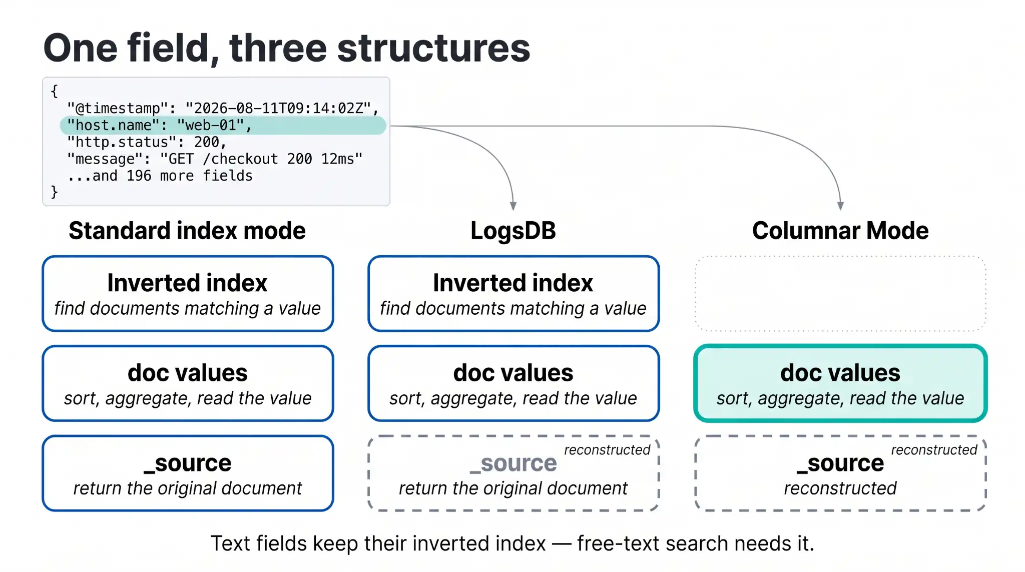
Doc values answer another question: "For this document, what are the values?" Doc values are laid out column by column so a scan touches only the bytes it needs. A flattened field uses both inverted indexes and doc values, so it can serve search and analytics from the same field.

The nature of the index means that the root field is only present in some cases. When the inverted index is disabled by the mapping, any value search requires a linear scan of the doc values for the searched value. In this case, when performing a search on the root field, there isn’t much additional overhead compared to just scanning the keyed field and ignoring the key markers. So the flattened mapper skips writing the root field, relying on the keyed field for both root and keyed queries.

Why flattened fields switched from dictionary to binary doc values

Historically, flattened field doc values used Lucene's SortedSetDocValues, which is a dictionary-compressed format. This means that every key\0value value indexed across all documents per segment is stored in one big sorted, deduplicated set of values. Each document tracks a list of ordinals into that value set.

This dictionary approach provides great compression for low-cardinality fields that tend to have repeated values. It is byte-efficient to store a value only once, and then refer to it by a single integer value. However, there is overhead associated with building and maintaining that dictionary of values, and that overhead is wasted effort when operating on high-cardinality fields that don’t repeat values.

Because flattened fields are a catch-all type, their cardinality tends to be very high. So while the dictionary approach works, it’s not the most compact or scan-friendly layout for this data, especially in time-series indices where flattened bags are common and storage pressure is real.

Recent versions switched the storage to use Lucene’s BinaryDocValues. This format just stores a literal binary blob for each document, which is compressed using Zstandard by our doc values codec when written to disk.

This new binary format provides an additional benefit: it allows us to maintain original array ordering without any overhead. Flattened fields support the mapping parameter preserve_leaf_arrays, which affects how multivalued fields are returned when using synthetic source. When configured to preserve_leaf_arrays: exact, returned values preserve the order, duplicates, and nulls from the original source value.

The dictionary encoding inherent to sorted-set doc values means the returned values are sorted, deduplicated, and de-nulled. To implement preserve_leaf_arrays, flattened fields have traditionally used an additional sidecar field, tracking the required metadata to reconstruct the original source value. However, the nature of binary doc values means that this sidecar field is no longer needed. The values are just stored and returned as indexed.

Limitations of schema on read with flattened fields

The limitations below follow from the keyword-only rule and the shared keyed field:

• No numeric, date, or Boolean typing on dynamic keys. 100 and "100" are the same term.

• No fuzzy, regexp, or wildcard on a specific subkey.

• No multi-fields (fields) or copy_to on the flattened field.

• A depth_limit (default 20) on how deeply nested the object can be.

If you need real typing for a known key, flattened now supports explicitly mapped subfields: you declare individual keys with real types under a properties block, and those keys are indexed by their own typed mapper instead of the keyed field. You get numeric ranges on labels.status_code, while everything else in labels stays dynamic and keyword-only. This is the escape hatch for the handful of keys you actually know about.

Schema on read: querying flattened field JSON keys in ES|QL

Search has supported flattened fields for years. ES|QL, the newer, piped query language built on a columnar compute engine, now reads flattened fields, too. Support began in the Technical Preview of Elasticsearch 9.5.0. It has two distinct pieces.

What ES|QL returns when you select a flattened field

ES|QL uses a dedicated data type for flattened fields, rather than folding it into keyword. When you select the root, you get the whole object back as a JSON string:

FROM logs | KEEP labels

labels:flattened
{"k8s.pod":"web-7f9","region":"us-east-1"}

Keys come back sorted. You can carry this value through a query, count it, group by it, and run the multi-value and comparison functions on it. But an opaque JSON blob is not usually what you want to filter or aggregate on. For that, you need to reach inside it and process its contents.

How FIELD_EXTRACT reads JSON keys from flattened fields

There is no dotted-path syntax for dynamic keys in ES|QL. You cannot write labels.region for an unmapped key, because to the engine the flattened root is a single leaf value, not a set of columns. Instead you use a function:

FROM logs
| EVAL region = FIELD_EXTRACT(labels, "region")
| STATS count = COUNT(*) BY region
| SORT region

The absence of a dotted-path syntax is a tentative limitation. The keyed field already addresses individual subkeys, so a more natural syntax for reaching into a flattened root is something we are planning to support.

FIELD_EXTRACT(field, path) takes a flattened field and a key, and returns a keyword. The rules are easier to see against a document. Take this one:

POST logs/_doc
{
 "labels": {
   "region": "us-east-1",
   "k8s": { "pod": "web-7f9", "node": "ip-10-0-0-3" },
   "tags": ["prod", "canary"],
   "retries": 4
 }
}

And this query:

FROM logs
| EVAL region    = FIELD_EXTRACT(labels, "region")
| EVAL pod       = FIELD_EXTRACT(labels, "k8s.pod")
| EVAL k8s       = FIELD_EXTRACT(labels, "k8s")
| EVAL tags      = FIELD_EXTRACT(labels, "tags")
| EVAL retries   = FIELD_EXTRACT(labels, "retries")
| EVAL namespace = FIELD_EXTRACT(labels, "k8s.namespace")

The result is:

region     | pod     | k8s  | tags            | retries | namespace
us-east-1  | web-7f9 | null | [prod, canary]  | 4       | null

Four things to take from this:

• The dot is part of the key, not a navigation operator. The mapper already collapsed the nested object into the flat key k8s.pod, so "k8s.pod is a direct lookup, not a walk from k8s to pod.

• Matching is exact. "k8s" returns null because there is no leaf stored at k8s, only at k8s.pod and k8s.node. For the same reason, "host" will not find "host.name", and matching is case-sensitive, so "Region" will not find "region".

• Arrays come back multi-valued. "tags" yields a multi-valued keyword you can MV_EXPAND, count, or filter on. A missing key yields null.

• Everything is a keyword. "retries" comes back as the string "4", and a Boolean leaf comes back as "true" or "false".

JSONPath syntax is rejected outright, at parse time rather than per row. Both FIELD_EXTRACT(labels, "['k8s.pod']") and FIELD_EXTRACT(labels, "tags[0]") fail with field_extract path must be a literal flattened sub-field name.

Once extracted, the value is an ordinary keyword column. You can filter on it, group by it, sort by it, or use it as the join key in a LOOKUP JOIN:

FROM logs
| EVAL host_name = FIELD_EXTRACT(resource.attributes, "host.name")
| LOOKUP JOIN host_info ON host_name

How ES|QL pushes flattened field predicates into the columnar store

The obvious way to implement FIELD_EXTRACT would be to read the whole flattened root out of storage, render it as a JSON string, hand it to the compute engine, and parse it once per row to pull out a single key. But that means reading every key to use once and paying for a JSON parse on every document. So this obvious implementation is not performant.

ES|QL avoids this whenever possible. Between storage and the compute engine sits the block loader, the step that turns stored data into the columnar blocks the engine operates on. FIELD_EXTRACT hooks into that step instead of running after it.

When ES|QL loads a column, the flattened field type inspects the request. If the request is an extraction of a single constant key and the field has doc values, it routes straight to the keyed doc-values loader, which reads the key\0value entries for only that key out of the columnar structure. The column that arrives at the compute engine already contains only that key's values. The JSON string is never built and never parsed, and the other keys in the object are never read.

When extraction can’t be fused into the block loader, for example, because the key is computed per row or the root is the output of another function such as CASE, ES|QL falls back to the parse-per-row path. The results are identical either way. Only the cost changes.

The comparison can push down further. A predicate like FIELD_EXTRACT(labels, "region") == "us-east-1" can be pushed to Lucene as a term query against the synthetic keyed field, the same region\0us-east-1 term the search path uses. So a filter on an extracted subkey can be answered by the inverted index (if available), and the projection can be answered by doc values, exactly like a first-class field, even though the key was never in the mapping.

Ordering comparisons push down, too. The four, single-sided comparators (>, >=, <, <=) and closed BETWEEN-style ranges all become a range query on that same synthetic keyed field. This is where the key\0 / key\1 sentinels earn their keep: the single-sided forms are only pushable because the mapper can box an open bound inside the key. The pushed range is treated as a candidate, and the predicate is re-evaluated on the extracted keyword column afterwards, so multi-valued keys don’t slip through.

The values are keywords, so the ordering is lexicographic, not numeric. FIELD_EXTRACT(labels, "retries") > "10" compares strings, which means "9" is greater than "10". If you need numeric ranges on a key, map it explicitly under properties, or cast the value in ESQL.

Explicitly mapped subfields behave differently on purpose. Because they carry real types, comparison semantics diverge from the keyword path, so they are loaded and compared through their own typed mapper rather than fused into the keyed loader. And when you select a flattened root that has mapped subfields, ES|QL loads it from _source, so every leaf renders as a string and no keys are dropped silently.

When to use flattened fields vs. dynamic mapping in Elasticsearch

Use flattened fields when:

• The set of keys is open-ended or unknown ahead of time.

• You would otherwise cause a mapping explosion.

• Keyword-level filtering and grouping on the values is enough, and you don’t need numeric or date semantics on the dynamic keys.

• You have a few keys that do need real types. Map those explicitly under properties, and let the rest stay dynamic.

Avoid it, or map fields normally, when the schema is stable and you need full-text analysis, numeric aggregation, or date math across the board.

Remember that flattened is not a dumping ground for JSON you have given up on. It’s a real columnar-and-inverted store for schemaless data, and with ES|QL support, it’s now a first-class analytical citizen. You can keep the messy, unmapped parts of your data messy, and still filter, group, join, and aggregate across them as needed.