Predicting flight delays with regression analysis
editPredicting flight delays with regression analysis
editLet’s try to predict flight delays by using the
sample flight data. The data set contains
information such as weather conditions, flight destinations and origins, flight
distance, carrier, and the number of minutes each flight was delayed. When you
create a data frame analytics job for regression analysis, it learns the relationships
between the fields in your data in order to predict the value of a
dependent variable, which in this case is the numeric FlightDelayMins field.
For an overview of these concepts, see Regression.
Preparing your data
editEach document in the sample flight data set contains details for a single flight, so this data is ready for analysis; it is already in a two-dimensional entity-based data structure. In general, you often need to transform the data into an entity-centric index before you analyze the data.
In order to be analyzed, a document must contain at least one field with a
supported data type (numeric, boolean, text, keyword or ip) and must
not contain arrays with more than one item. If your source data consists of some
documents that contain the dependent variable and some that do not, the model is
trained on the subset of the documents that contain it.
Example source document
{
  "_index": "kibana_sample_data_flights",
  "_type": "_doc",
  "_id": "S-JS1W0BJ7wufFIaPAHe",
  "_version": 1,
  "_seq_no": 3356,
  "_primary_term": 1,
  "found": true,
  "_source": {
    "FlightNum": "N32FE9T",
    "DestCountry": "JP",
    "OriginWeather": "Thunder & Lightning",
    "OriginCityName": "Adelaide",
    "AvgTicketPrice": 499.08518599798685,
    "DistanceMiles": 4802.864932998549,
    "FlightDelay": false,
    "DestWeather": "Sunny",
    "Dest": "Chubu Centrair International Airport",
    "FlightDelayType": "No Delay",
    "OriginCountry": "AU",
    "dayOfWeek": 3,
    "DistanceKilometers": 7729.461862731618,
    "timestamp": "2019-10-17T11:12:29",
    "DestLocation": {
      "lat": "34.85839844",
      "lon": "136.8049927"
    },
    "DestAirportID": "NGO",
    "Carrier": "ES-Air",
    "Cancelled": false,
    "FlightTimeMin": 454.6742272195069,
    "Origin": "Adelaide International Airport",
    "OriginLocation": {
      "lat": "-34.945",
      "lon": "138.531006"
    },
    "DestRegion": "SE-BD",
    "OriginAirportID": "ADL",
    "OriginRegion": "SE-BD",
    "DestCityName": "Tokoname",
    "FlightTimeHour": 7.577903786991782,
    "FlightDelayMin": 0
  }
}
The sample flight data set is used in this example because it is easily accessible. However, the data has been manually created and contains some inconsistencies. For example, a flight can be both delayed and canceled. This is a good reminder that the quality of your input data affects the quality of your results.
Creating a regression model
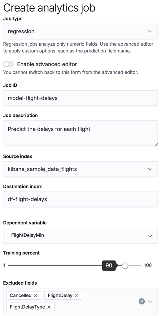
editTo predict the number of minutes delayed for each flight:
-
Create a data frame analytics job.
You can use the wizard on the Machine Learning > Data Frame Analaytics tab in Kibana or the create data frame analytics jobs API.
-
Choose
regressionas the job type. -
Choose
kibana_sample_data_flightsas the source index. - Add the name of the destination index that will contain the results of the analysis. It will contain a copy of the source index data where each document is annotated with the results. If the index does not exist, it will be created automatically.
-
Choose
FlightDelayMinas the dependent variable, which is the field that we want to predict with the regression analysis. -
Choose a training percent of
90which means it randomly selects 90% of the source data for training. -
Add
Cancelled,FlightDelay, andFlightDelayTypeto the list of excluded fields. These fields will be excluded from the analysis. It is recommended to exclude fields that either contain erroneous data or describe thedependent_variable. - Use the default memory limit for the job. If the job requires more than this amount of memory, it fails to start. If the available memory on the node is limited, this setting makes it possible to prevent job execution.
API example
PUT _ml/data_frame/analytics/model-flight-delays { "source": { "index": [ "kibana_sample_data_flights" ], "query": { "range": { "DistanceKilometers": { "gt": 0 } } } }, "dest": { "index": "df-flight-delays" }, "analysis": { "regression": { "dependent_variable": "FlightDelayMin", "training_percent": 90 } }, "analyzed_fields": { "includes": [], "excludes": [ "Cancelled", "FlightDelay", "FlightDelayType" ] } } -
Choose
-
Start the job in Kibana or use the start data frame analytics jobs API.
The job takes a few minutes to run. Runtime depends on the local hardware and also on the number of documents and fields that are analyzed. The more fields and documents, the longer the job runs. It stops automatically when the analysis is complete.
API example
POST _ml/data_frame/analytics/model-flight-delays/_start
-
Check the job stats to follow the progress in Kibana or use the get data frame analytics jobs statistics API.
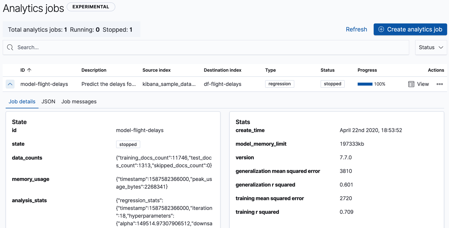
The job has four phases (reindexing, loading data, analyzing, and writing results). When all the phases have completed, the job stops and the results are ready to view and evaluate.
API example
GET _ml/data_frame/analytics/model-flight-delays/_stats
The API call returns the following response:
{
  "count" : 1,
  "data_frame_analytics" : [
    {
      "id" : "model-flight-delays",
      "state" : "stopped",
      "progress" : [
        {
          "phase" : "reindexing",
          "progress_percent" : 100
        },
        {
          "phase" : "loading_data",
          "progress_percent" : 100
        },
        {
          "phase" : "analyzing",
          "progress_percent" : 100
        },
        {
          "phase" : "writing_results",
          "progress_percent" : 100
        }
      ],
      "data_counts" : {
        "training_docs_count" : 11746,
        "test_docs_count" : 1313,
        "skipped_docs_count" : 0
      },
      "memory_usage" : {
        "timestamp" : 1587582366000,
        "peak_usage_bytes" : 2268341
      },
      "analysis_stats" : {
        "regression_stats" : {
          "timestamp" : 1587582366000,
          "iteration" : 18,
          "hyperparameters" : {
            "alpha" : 149514.97307906512,
            "downsample_factor" : 0.9598240037838769,
            "eta" : 0.02331774683318901,
            "eta_growth_rate_per_tree" : 1.0143154178910303,
            "feature_bag_fraction" : 0.5504020748926737,
            "gamma" : 59.759601447901105,
            "lambda" : 0.9196397223419859,
            "max_attempts_to_add_tree" : 3,
            "max_optimization_rounds_per_hyperparameter" : 2,
            "max_trees" : 894,
            "num_folds" : 4,
            "num_splits_per_feature" : 75,
            "soft_tree_depth_limit" : 4.7434397922600615,
            "soft_tree_depth_tolerance" : 0.13448633124842999
          },
          "timing_stats" : {
            "elapsed_time" : 568868,
            "iteration_time" : 21377
          },
          "validation_loss" : {
            "loss_type" : "mse",
            "fold_values" : [ ]
          }
        }
      }
    }
  ]
}
Viewing regression results
editNow you have a new index that contains a copy of your source data with predictions for your dependent variable.
When you view the regression results in Kibana, it shows the contents of the destination index in a tabular format:
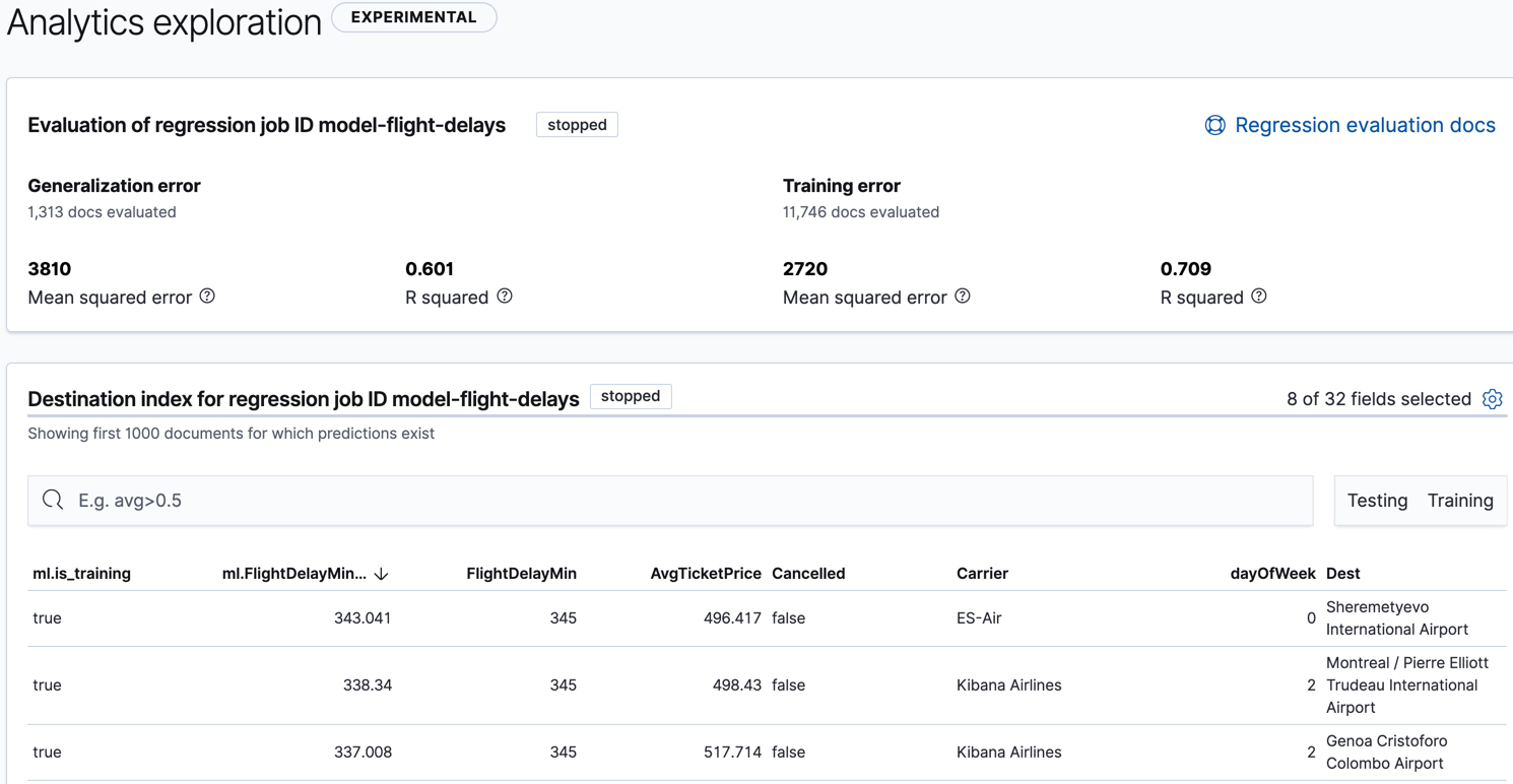
In this example, the table shows a column for the dependent variable
(FlightDelayMin), which contains the ground truth values that we are trying to
predict with the regression analysis. It also shows a column for the prediction values
(ml.FlightDelayMin_prediction) and a column that indicates whether the
document was used in the training set (ml.is_training). You can filter the
table to show only testing or training data and you can select which fields are
shown in the table.
If you do not use Kibana, you can see the same information by using the standard Elasticsearch search command to view the results in the destination index.
API example
GET df-flight-delays/_search
The snippet below shows a part of a document with the annotated results:
          ...
          "DestRegion" : "UK",
          "OriginAirportID" : "LHR",
          "DestCityName" : "London",
          "FlightDelayMin" : 66,
          "ml" : {
            "FlightDelayMin_prediction" : 62.527,
            "is_training" : false
          }
          ...
Evaluating regression results
editThough you can look at individual results and compare the predicted value
(ml.FlightDelayMin_prediction) to the actual value (FlightDelayMins), you
typically need to evaluate the success of the regression model as a whole.
Kibana provides training error metrics, which represent how well the model performed on the training data set. It also provides generalization error metrics, which represent how well the model performed on testing data.
A mean squared error (MSE) of zero means that the models predicts the dependent variable with perfect accuracy. This is the ideal, but is typically not possible. Likewise, an R-squared value of 1 indicates that all of the variance in the dependent variable can be explained by the feature variables. Typically, you compare the MSE and R-squared values from multiple regression models to find the best balance or fit for your data.
For more information about the interpreting the evaluation metrics, see Regression evaluation.
You can alternatively generate these metrics with the data frame analytics evaluate API.
API example
POST _ml/data_frame/_evaluate
{
 "index": "df-flight-delays",
  "query": {
      "bool": {
        "filter": [{ "term":  { "ml.is_training": true } }]
      }
    },
 "evaluation": {
   "regression": {
     "actual_field": "FlightDelayMin",
     "predicted_field": "ml.FlightDelayMin_prediction",
     "metrics": {
       "r_squared": {},
       "mean_squared_error": {}
     }
   }
 }
}
|
The destination index which is the output of the data frame analytics job. |
|
|
Calculate the training error by evaluating only the training data. |
|
|
The field that contains the actual (ground truth) value. |
|
|
The field that contains the predicted value. |
The API returns a response like this:
{
  "regression" : {
    "mean_squared_error" : {
      "error" : 2720.148614307912
    },
    "r_squared" : {
      "value" : 0.7087320824507466
    }
  }
}
Next, we calculate the generalization error:
POST _ml/data_frame/_evaluate
{
 "index": "df-flight-delays",
  "query": {
      "bool": {
        "filter": [{ "term":  { "ml.is_training": false } }]
      }
    },
 "evaluation": {
   "regression": {
     "actual_field": "FlightDelayMin",
     "predicted_field": "ml.FlightDelayMin_prediction",
     "metrics": {
       "r_squared": {},
       "mean_squared_error": {}
     }
   }
 }
}
If you don’t want to keep the data frame analytics job, you can delete it. For example, use Kibana or the delete data frame analytics job API. When you delete data frame analytics jobs, the destination indices remain intact.