Querying a petabyte of cloud storage in 10 minutes
Elastic's new frozen data tier decouples compute from storage and leverages low-cost object stores such as Google Cloud Storage, Azure Blob Storage, or Amazon S3 to directly power searches. It provides unlimited scaling of storage while preserving the ability to efficiently query the data without any need to rehydrate it first, making it easier and cheaper to manage data at scale.
In this blog post we compare search performance on the new frozen tier with the existing Elasticsearch data tiers, and we show how with the frozen tier you can store and search far larger amounts of data at lower performance. The main highlights of the frozen tier are:
- Return results from a simple term query over a 4TB dataset in just a couple of seconds if the data isn’t cached. If it’s cached, the performance is in the milliseconds — similar to the warm or cold tiers.
- Computing a complex Kibana dashboard over the 4TB data set completes in under five minutes if the data isn’t cached. If it’s cached, it completes in a few seconds — similar to the warm or cold tiers.
- Easily scale up your data volume to a 1PB dataset. Uncached, the results of a simple term query will return in under 10 minutes.
The frozen tier is currently available as a technical preview in Elasticsearch 7.12 and on Elastic Cloud, and will be generally available soon.
A quick introduction to data tiers
Data tiers provide optimized storage and processing power for accessing data based on various needs, for example based on age, data source, or some other criteria. The hot tier typically handles all indexing of new data in the cluster and holds the most recent daily indices that tend to be queried most frequently. As indexing is often an I/O-intensive activity, the hardware these nodes run on needs to be more powerful and therefore uses SSD storage. The warm tier can handle larger amounts of indices that are less frequently queried, and can therefore instead use cheaper storage with longer latency, such as very large spinning disks, reducing the overall cost of retaining data over time yet making it still accessible for queries.
The recently introduced cold and frozen data tiers leverage low-cost object stores to cost-effectively manage large data volumes while still having the ability to search on them.
The cold tier eliminates the need for replicas, powering recovery events by restoring the data from a snapshot instead. In the hot and warm tiers, half of the disk space is typically used to store replica shards. These redundant copies ensure fast and consistent query performance and provide resilience in case of machine failures, where a replica takes over as the new primary. Once the data becomes read-only in its lifecycle, however, recovery can be offloaded to a snapshot. This means that in the cold tier, replica shards are not needed; in case a node or disk fails, the data is automatically recovered from a snapshot, recreating a full copy in the cluster so that searches can be served from local disks again. The snapshot repository is a perfect fit for this, since it's much cheaper to store data in a blob store than on either local SSDs or spinning disks, and in most cases, the data is already in the blob store anyway for backup purposes. The cold tier therefore only needs half of the local storage space of the warm tier, having similar query performance and only slightly worse availability, providing a 50% cost savings over the warm tier.
The frozen tier takes this one step further, decoupling compute from storage by only caching small but frequently accessed parts of the data locally in the cluster and lazily fetching the data from the object store, on an as-needed basis, as searches require them. This provides much higher compute to storage ratios than what's been possible so far with Elasticsearch. Searches in this frozen tier are of course potentially much slower than in the hot, warm, or cold tiers, but this can be an acceptable tradeoff for less frequent searches such as operational or security investigations, legal discoveries, or historical performance comparisons. The advantage of having everything indexed by default in Elasticsearch makes this feature very powerful, as it avoids doing a full scan of the data at query time, and leverages these index structures to quickly return results over very large data sets.
How the frozen tier works
A node in the frozen tier does not need to have enough disk space for a full copy of all its indices. Instead we have introduced an on-disk LFU cache which caches only portions of the index data downloaded from the blob store to serve a given query. The on-disk cache works similarly to the operating system's page cache, speeding up access to frequently requested parts of the blob store data. Read requests at the Lucene level are mapped to read requests on this local cache. In case of a cache miss, a larger region of the Lucene file (16MB chunk) is downloaded from the blob store and made available to the search. The next time that this same region of the file is accessed by Lucene, it is served straight from the local cache.
The node-level shared cache evicts mapped file regions based on a "least-frequently-used" policy, as we expect some regions of the Lucene files to be used more frequently than other regions. If some regions of a Lucene file are needed to answer queries over and over (such as range queries on the @timestamp field) that data will remain cached while other data might be evicted.
While searches now require downloading regions of the files that are being accessed, Lucene's way of executing searches based on a precomputed set of index structures reduces the amount of data to scan and makes this fast. To further reduce the memory footprint of these shards, we only open up the Lucene index on demand, that is, whenever there's an active search. This gives us the ability to have a large number of indices on a frozen tier node.
Benchmarking goals
For each tier, we measure search performance upon first access (not leveraging any caches, as they haven't been warmed up yet), as well as repeat searches with the same query (caches warmed up). For the frozen tier, we also check repeat search performance when the on-disk LFU cache can't fit all the data.
We consider two types of queries for this benchmark. The first is representative of a security investigation, finding a small set of matching documents in a large data set (needle in a haystack), and the second one represents a Kibana dashboard that is computing multiple heavy aggregations over large amounts of data.
As the goal of these benchmarks is to accurately compare query performance across different tiers, we’ve elected to use the same machine type across all of them; in a real deployment, however, tier-specific machine types should be used, trading off optimal cost and performance per tier. The baseline in our benchmark is the hot tier where we have regular time-based Elasticsearch indices. As the warm tier is accessing data in the same way as the hot tier, and we are using the same machine type across all tiers here for the purposes of this benchmark, it is equivalent to the hot tier and not listed separately. In the cold tier, we have a full copy of those same indices mounted from a snapshot. In the frozen tier, we have indices mounted from a snapshot using the on-disk LFU cache.
Benchmark setup
The benchmarks are run on Google Cloud using Elasticsearch 7.12.1, and are based on an event-based data set of web server logs that Elastic is using for benchmarking various features. The size of the indexed data set on disk is 4TB (10 time-based indices with 5 shards of 80GB each and 35 fields in each mapping). Shards are force-merged down to one segment, which optimizes for read performance, and which is the default that index lifecycle management uses when moving data to the frozen tier. The same (precomputed) snapshot of the data, accessed in Google Cloud Storage using Elasticsearch's repository-gcs plugin, is used to benchmark each tier. Recovery throttling is disabled to not artificially limit the performance.
The first search that we benchmark is just a simple term query that finds occurrences in the data set where a given IP address has accessed the web server, "nginx.access.remote_ip": "1.0.4.230".
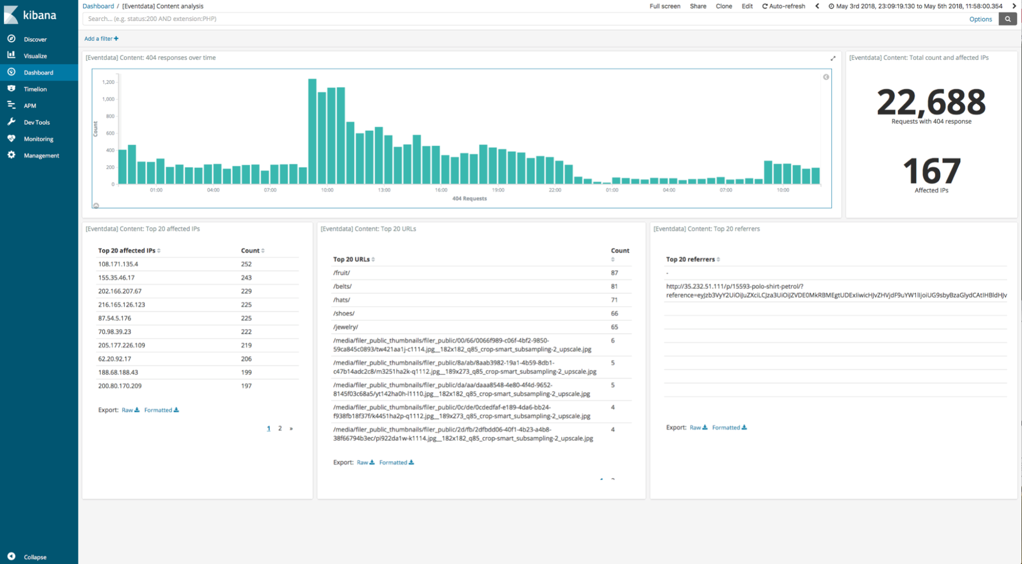
The second search is a Kibana dashboard that contains five visualisations and is designed to be used for analysis of requests with a 404 response code — for example, to find links that are no longer leading anywhere.
Before each benchmark scenario we run a number of preparatory steps to reduce run-to-run variation, including dropping OS caches and slab objects and trimming the SSD disks. On the hot/warm tier, Elasticsearch uses the hybridfs store type as default, which memory maps some of the Lucene file types. The cold and frozen tiers do not use memory mapping. As memory mapping has effects on the page cache by prefetching pages, we provide both the results in the hot/warm tier when using memory mapping, as well as when configuring it with the "niofs" index.store.type, which is closer to how we access the local files in the cold and frozen tiers.
For simplicity we benchmark only a single-node cluster here, but each tier also supports multi-node clusters. The single-node cluster is an N2D (n2d-custom-8vCPUs-64GB) instance on Google Cloud with 8 vCPUs, 64GB RAM (29GB of which is used by Elasticsearch for JVM heap), and 16x375GB local scratch SSD disks in RAID-0 so that it can fit the full 4TB data set in the hot/warm and cold tiers. It is a suitable candidate instance for frozen as it has fast local disks for the on-disk LFU cache and a fast network connection to Google Cloud Storage.
We also experiment with two different cache sizes for the on-disk LFU cache in the frozen tier to show its importance for repeat searches: 200GB (5% of data set) and 20GB (0.5% of data set).
Results
Query performance is impacted by various caching mechanisms, from the OS-level page cache to application-level in-memory caches such as the shard request cache and the node query cache in Elasticsearch. For each of the results, we explain how these caches come into play. The results shown are median values of five runs in order to reduce run-to-run variation.
Simple term query
Let's start with the simple term query. The main observation here is that the frozen tier returns the results (5 matching documents) over the 4TB data set within a few seconds, downloading only a tiny portion of the data set to find matching elements. This highlights the power of the index structures in Lucene that allow this fast lookup.
Repeat runs of the query show comparable performance across all tiers, as the data can now be served in the frozen tier from the local on-disk LFU cache. Elasticsearch's in-memory result caches do not come into play here, as this type of query is not cached. Performance of repeat runs in the hot/warm and cold tier is impacted by having the data available in the page cache.
Simple term query on 4TB data set | |||
Action | Hot/warm tier niofs | Cold tier | Frozen tier |
Simple term query: first run | 92ms | 95ms | 6257ms |
Simple term query: repeat run | 29ms | 38ms | 76ms |
Note: The same machine type is used in all tiers to demonstrate query improvement from cache reuse on the frozen tier. This is not query performance across different tiers in real deployments. See benchmark goals for more details.
Performance in the hot/warm tier is slightly lower on first run when using the default index store type hybridfs instead of niofs (285ms instead of 92ms), with more details in the following section.
Kibana dashboard
We repeat the same process for the Kibana dashboard. The main observation here is that the frozen tier returns the dashboard over the same 4TB data set within 5 minutes, compared to the 20 seconds it takes for the dashboard to be computed in the other tiers with local data access. Even though the dashboard is aggregating over 75% of the data set using a time-range filter, it still only needs to download a fraction of the data in the repository thanks to the index structures (approximately 3% in this case, as follows below in more detail).
Kibana dashboard on 4TB data set | ||||
Action | Hot/warm tier niofs | Cold tier | Frozen tier (5% cache) | Frozen tier (0.5% cache) |
Dashboard: first run | 16.3s | 16.6s | 282.8s | 321.5s |
Dashboard: exact repeat run without ES result caches | 6.2s | 7.1s | 11.1s | 224.1s |
Dashboard: exact repeat run with ES result caches | 80ms | 75ms | - | - |
Dashboard: similar repeat run without ES result caches | 19.5s | 20.3s | 23.4s | 238.4s |
When Elasticsearch's result caches are disabled, the performance of repeat searches mainly depends on the page cache, and are comparable in performance with the frozen tier when the portions of the data needed for the query fully fits into the on-disk LFU cache. Interesting to observe here as well is that, for this particular workload, memory mapping in the hot/warm tier is causing page cache thrashing which negatively impacts performance of the hot/warm tier when using the default store type (up to three times slower compared to 6.2s with niofs).
For the frozen tier, we consider two different sizes for the LFU cache to show the effect on repeat search performance. The on-disk LFU cache is first dimensioned to 200GB, which is only a fraction of the 4TB (5% of the data set's size), but still big enough to hold all the data that has been downloaded to compute the given dashboard (approximately 3%, or 120GB). In a second benchmarking run, it's dimensioned to only 20GB (0.5% of the original data set's size), which isn't enough to hold all the data for the given dashboard.
When Elasticsearch's in-memory caches are enabled, repeat searches are even faster, as parts of the query results are now directly available on the Elasticsearch node and do not need to be recomputed. However, currently the frozen tier does not use these in-memory Elasticsearch caches.
We have also benchmarked the case where only a slightly different dashboard is computed, filtering by a different country code. In this case the frozen tier can benefit from having already downloaded many portions of the data that are relevant to satisfy this slightly different query, and returns results nearly as fast as the other tiers.
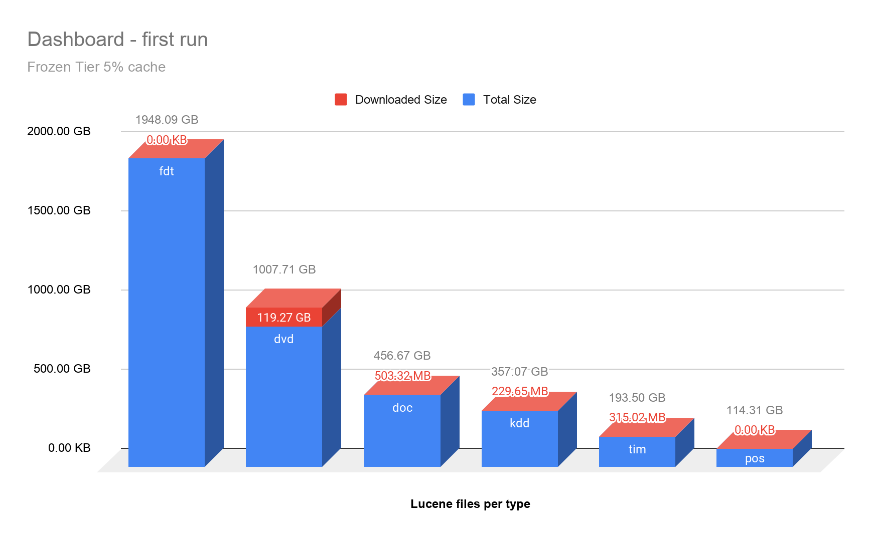
To show what's been downloaded in the frozen tier during the first run of the dashboard, we have visualized the six largest Lucene file types requested, as well as how much of them has been downloaded. While fdt (Field Data) files consume the most space (storing the documents), those are not accessed to compute aggregations. As expected, most of the access is done on Lucene's dvd (Per-Document Values) files, the doc values that are used for aggregating.
Fast access to large amounts of object storage
While querying on the frozen tier is certainly slower, its main benefit is for infrequent access where the data does not need to be rehydrated to be available for search. In comparison, making the full data set available locally would take more than an hour, even with recovery throttling disabled, which is far longer than it took us to directly run queries on the frozen tier.
Making 4TB data set accessible | |||
Action | Hot/warm tier | Cold tier | Frozen tier |
Restore indices from snapshot | 72.4min | - | - |
Mount indices from snapshot | - | 115s | 47s |
Prewarming (time for data to be fully available locally in the cold tier) | - | 82.8min | - |
Scaling to a petabyte
The benchmarks so far focused on comparative performance between the tiers, but couldn't show the full scale of what's possible with the frozen tier. This tier provides higher compute to storage ratios than the other tiers. To push this a bit to the extreme we've mounted the same data set from above 250 times, each time under a different name so that it's treated as separate indices. Our single-node cluster then had 12500 shards of 80GB each, which amounts to exactly one petabyte (1PB) of data mounted. Running the simple term query on that full 1PB (= 1 million GB) data set took less than 10 minutes, showing how well the implementation scales to larger data sets.
Simple term query on 1PB data set | |||
Action | Hot/warm tier | Cold tier | Frozen tier |
Simple term query: first run | Not possible (would need 1PB of local storage!) | 554s | |
Simple term query: repeat run (with 4TB on-disk LFU cache) | 127s | ||
In practice, this might not make for an ideal setup with such a large number of shards on a single node and an extremely low ratio of local disk cache versus object storage size. At this scale, the storage costs for the data set also dwarf the compute costs for the frozen tier node, so adding more nodes would significantly benefit performance while having a negligible impact on cost.
Sizing the on-disk LFU cache
As we've previously seen, dimensioning the on-disk LFU cache matters in order to achieve good performance for repeat searches. Here the right value very much depends on the kind of queries that are run, in particular how much data needs to be accessed to yield the query results. Having larger amounts of data mounted therefore does not necessarily always require a larger on-disk cache. Applying a time range filter, for example, in the context of time-based indices reduces the number of shards that need to be queried. As there is often some kind of underlying spatial or temporal locality in data access patterns, the frozen tier will allow efficient querying on very large data sets. Based on our current observations we recommend sizing the on-disk LFU cache so that it's between 1% and 10% of the mounted data set's size. A ratio of 5% is perhaps a good starting point for experimentation.
Note that both vertical as well as horizontal scaling is well supported by the frozen tier, as the computations are of a very parallel nature. Just using more performant machine types or adding more nodes to the cluster is a simple way to increase query performance on the frozen tier.
Conclusion
We have shown that the frozen tier can respond to two different types of queries with great performance. With Elasticsearch's index-by-default strategy, search performance in the frozen tier is orders of magnitude faster than scanning over the full data set. Repeat searches in the frozen tier further benefit from the on-disk cache and provide similar performance as the other tiers.
The frozen tier provides great value when cost-effective storage coupled with flexible compute to storage ratios is the main objective. The data in the frozen tier is just accessed as any regular index, making it easy to switch an existing setup to make use of this new exciting feature. Setting it up is also not difficult, as it's reusing snapshot repositories which are already used for backup purposes, and has full integration into index lifecycle management to transition data from hot/warm/cold to the frozen tier. Kibana's async search integration provides extended capabilities on top of this, allowing slow running dashboards to be computed in the background, and visualized when available.
The frozen tier is both available for self-hosted deployments as well as on Elastic Cloud, so check out the documentation, give it a try, and provide us your feedback.