Improving search relevance with data-driven query optimization
When building a full-text search experience such as an FAQ search or Wiki search, there are a number of ways to tackle the challenge using the Elasticsearch Query DSL. For full-text search there’s a relatively long list of possible query types to use, ranging from the simplest match query up to the powerful intervals query.
Independent of the query type you choose, you’ll also be faced with understanding and tweaking a list of parameters. While Elasticsearch uses good defaults for query parameters, they can be improved based on the documents in the underlying index (the corpus) and the specific kinds of query strings users will search with. To tackle this task, this post will walk you through the steps and techniques of optimizing a query following a structured and objective process.
Before we jump in, let’s consider this example of a multi_match query which searches for a query string on two fields of a document.
GET /_search
{
  "query": {
    "multi_match": {
      "query": "this is a test",
      "fields": [ "subject^3", "message" ]
    }
  }
}
Here we’re using the field boost parameter to specify that scores with matches on the subject field should be boosted and multiplied by a factor of three. We do this in an attempt to improve the overall relevance of the query — documents that are the most meaningful with respect to the query should be as close to the top of the results as possible. But how do we choose an appropriate value for the boost? How can we set the boost parameter for not just two fields but a dozen fields?
The process of relevance tuning is about understanding the effects of these various parameters. Of all the parameters you could tweak and tune, which ones should you try, with which values, and in which order? While a deep understanding of scoring and relevance tuning shouldn’t be ignored, how can we take a more principled approach to optimizing our queries? Can we use data from user clicks or explicit feedback (e.g., a thumbs up or down on a result) to drive tuning query parameters to improve search relevance? We can, so let’s dive in!
To accompany this blog post we’ve put together some example code and Jupyter notebooks that walk you through the steps of optimizing a query with the techniques outlined below. Read this post first, then head over to the code and see all the pieces in action. As of the writing of this post we’re using Elasticsearch 7.10 and everything should work with any of the Elasticsearch licenses.
Introducing MS MARCO
To better explain the principles and effects of query parameter tuning, we’re going to be using a public dataset called MS MARCO. The MS MARCO dataset is a large dataset curated by Microsoft Research containing 3.2 million documents scraped from web pages and over 350,000 queries sourced from real Bing web search queries. MS MARCO has a few sub-datasets and associated challenges, so we’re going to focus specifically on the document ranking challenge in this post, as it fits most closely with traditional search experiences. The challenge is effectively to provide the best relevance ranking for a set of selected queries from the MS MARCO dataset. The challenge is open to the public and any researcher or practitioner can participate by submitting their own attempts to come up with the best possible relevance ranking for a set of queries. Later in the post, you’ll see how successful we were by using the techniques outlined here. For the current standings of submissions, you can check out the official leaderboard.
Datasets and tools
Now that we have a rough goal in mind of improving relevance by tuning query parameters, let’s have a look at the tools and datasets that we’re going to be using. First let’s outline a more formal description of what we want to achieve and the data we will need.
- Given a:
- Corpus (documents in an index)
- Search query with parameters
- Labeled relevance dataset
- Metric to measure relevance
- Find: Query parameter values that maximize the chosen metric
Labeled relevance dataset
Right about now you might be thinking, “wait wait wait, just what exactly is a labeled relevance dataset and where do I get one?!” In short, a labeled relevance dataset is a set of queries with results that have been labeled with a relevance rating. Here’s an example of a very small dataset with just a single query in it:
{
  "id": "query1",
  "value": "tuning Elasticsearch for relevance",
  "results": [
    { "rank": 1, "id": "doc2", "label_id": 2, "label": "relevant" },
    { "rank": 2, "id": "doc1", "label_id": 3, "label": "very relevant" },
    { "rank": 3, "id": "doc8", "label_id": 0, "label": "not relevant" },
    { "rank": 4, "id": "doc7", "label_id": 1, "label": "related" },
    { "rank": 5, "id": "doc3", "label_id": 3, "label": "very relevant" }
  ]
}
In this example, we’ve used the relevance labels: (3) very relevant, (2) relevant, (1) related, and (0) not relevant. These labels are arbitrary and you may choose a different scale but the four labels above are pretty common. One way to get these labels is to source them from human judges. A bunch of people can look through your search query logs and for each of the results, provide a label. This can be quite time consuming so many people opt to collect this data from their users directly. They log user clicks and use a click model to convert click activity into relevance labels.
The details of this process are well beyond the scope of this blog post but have a look around for presentations and research on click models123. A good place to start is to collect click events for analytics purposes and then look at click models once you have enough behavioural data from users. Have a look at the recent blog post Analyzing online search relevance metrics with Elasticsearch and the Elastic Stack for more.
MS MARCO document dataset
As discussed in the introduction, for the purposes of demonstration we’re going to be using the MS MARCO document ranking challenge and associated dataset which has everything we need: a corpus and a labeled relevance dataset.
MS MARCO was first built to serve the purpose of benchmarking question and answer (Q&A) systems and all the queries in the dataset are actually questions of some form. For example, you won’t find any queries that look like typical keyword queries like “rules Champions League”. Instead, you will see query strings like “What are the rules of football for the UEFA Champions League?”. Since this is a question answering dataset, the labeled relevance dataset also looks a bit different. Since questions typically have just one best answer, the results have just one “relevant” label (1) and nothing else. Documents are pretty simple and consist of just three fields: url, title, body. Here’s an example (snippet) of a document:
- ID: D2286643
- URL: http://www.answers.com/Q/Why_is_the_Manhattan_Proj...
- Title: Why is the Manhattan Project important?
- Body: Answers.com ® Wiki Answers ® Categories History, Politics & Society History War and Military History World War 2 <snip> It was the 2nd most secret project of the war (cryptographic work was the 1st). It was the highest priority project of the war, the codeword "silverplate" was assigned to it and overrode all other wartime priorities. It cost $2,000,000,000. <snip> Edit Mike M 656 Contributions Answered In US in WW2 Why was the Manhattan project named Manhattan project? The first parts of the Manhattan project took part in the basement of a building located in Manhattan. Edit Pat Shea 3,370 Contributions Answered In War and Military History What is secret project of the Manhattan project? The Manhattan Project was the code name for the WWII project to build the first Nuclear Weapon, the Atomic Bomb. Edit
As you can see, documents have been cleaned and HTML markup has been removed, however they can sometimes contain all sorts of metadata. This is particularly true for user generated content as we see above.
Measuring search relevance
Our goal in this blog post is to establish a systematic way to tune query parameters to improve the relevance of our search results. In order to measure how well we are doing with respect to this goal, we need to define a metric that captures how well the results from a given search query satisfy a user’s needs. In other words, we need a way to measure relevance. Luckily we have a tool for this already in Elasticsearch called the Rank Evaluation API. This API allows us to take the datasets outlined above and calculate one of many search relevance metrics.
In order to achieve this, the API executes all of the queries from the labeled relevance dataset and compares the results from each query to the labeled results to calculate a relevance metric, such as precision, recall, or mean reciprocal rank (MRR). In our case the MS MARCO document ranking challenge has already selected the mean reciprocal rank (MRR) on the top 100 results (MRR@100) as the relevance metric. This makes sense for a question and answer dataset as MRR only cares about the first relevant document in a result set. It takes the reciprocal rank (1 / rank) of the first relevant document and averages them over all the queries.
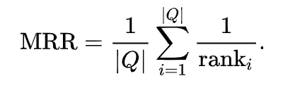
For the visually inclined, here’s an example calculation of MRR for a small set of queries:
Search templates
Now that we’ve established how we’d like to measure relevance with the help of the Rank Evaluation API, we need to look at how to expose query parameters to allow us to try different values. Recall from our basic multi_match example in the introduction how we set the boost value on the subject field.
GET /_search
{
  "query": {
    "multi_match": {
      "query": "this is a test",
      "fields": [ "subject^3", "message" ]
    }
  }
}
When we use the Rank Evaluation API, we specify the metric, the labeled relevance dataset, and optionally the search templates to use for each query. The method we’ll describe below is actually quite powerful since we can rely on search templates. Effectively, we can turn anything that we can parameterize in a search template into a parameter that we can optimize. Here’s another multi_match query but using the real fields from the MS MARCO document dataset and exposing a boost parameter for each.
{
  "query": {
    "multi_match": {
      "query": "{{query_string}}",
      "fields": [
        "url^{{url_boost}}",
        "title^{{title_boost}}",
        "body^{{body_boost}}"
      ]
    }
  }
}
The query_string will be replaced when we run the Rank Evaluation API, but these other boost parameters will be set every time we want to test new parameter values. If you are using queries with different parameters, like a tie_breaker, you can use the same templating to expose the parameter. Check out the search templates documentation for more details.
Parameter optimization: Putting it all together
Ok stay with me here! It’s finally time to put all these pieces together. We’ve seen each of the necessary components:
- Corpus
- Labeled relevance dataset
- Metric to measure relevance
- Search template with parameters
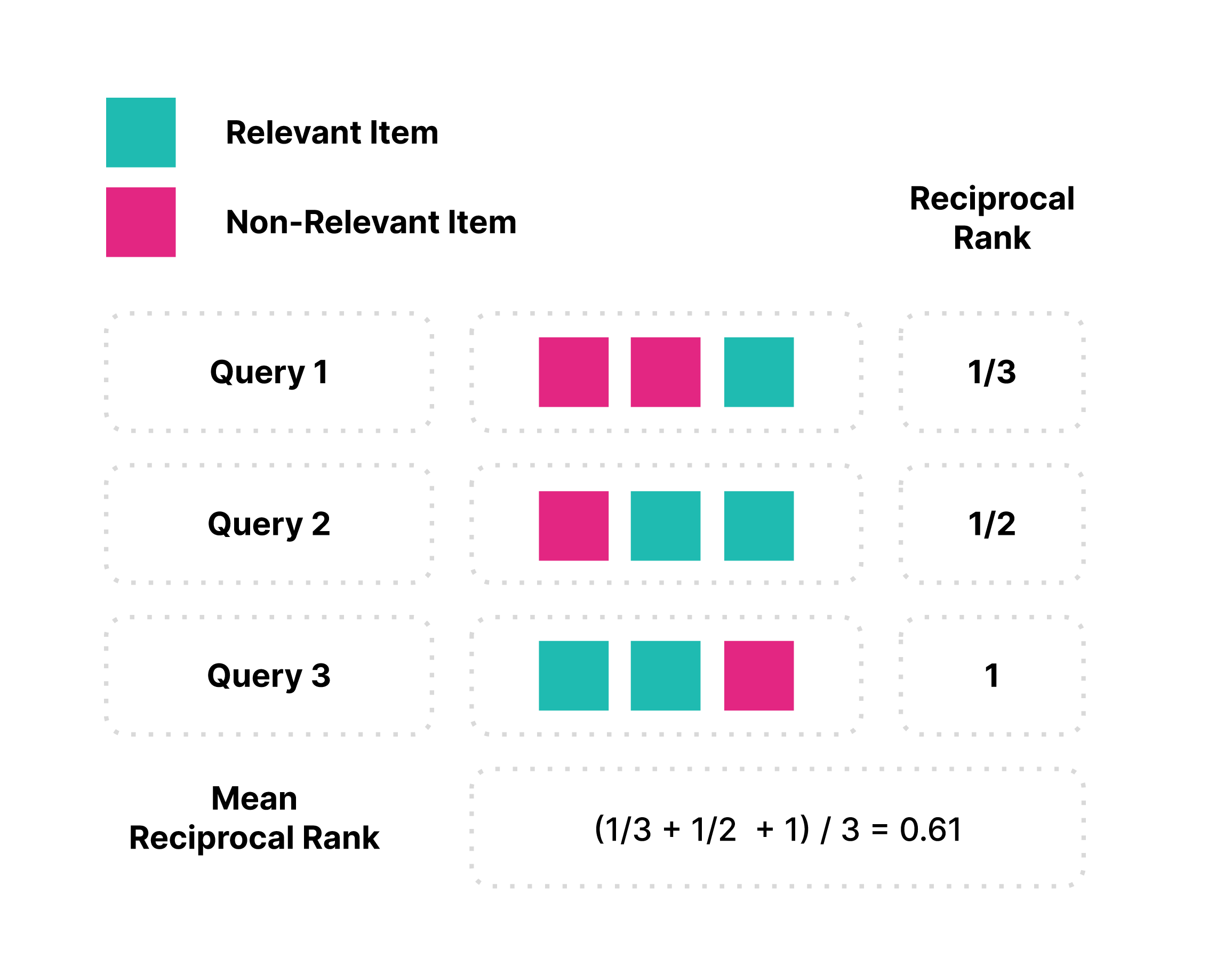
For this example we’re going to stitch all of this together using a Python script to submit requests to the Rank Evaluation API and orchestrate the workflow. The workflow is pretty simple: submit a Rank Evaluation API call with some parameter values to try, get the metric score (MRR@100), record the parameter values that produced that metric score, and iterate by picking new parameter values to try. At the end, we return the parameter values that produced the best metric score. This workflow is a parameter optimization procedure in which we’re maximizing the metric score.
In the workflow in Figure 3, we can see where all our datasets and tools are used, with the Rank Evaluation API taking center stage to run the queries and measure relevance by the provided metric. The only thing we haven’t touched on yet is how to pick the parameter values to try in each iteration. In the following sections, we’ll discuss two different methods for picking parameter values: grid search and Bayesian optimization. Before we talk about methods though, we need to introduce the concept of a parameter space.
Parameter spaces
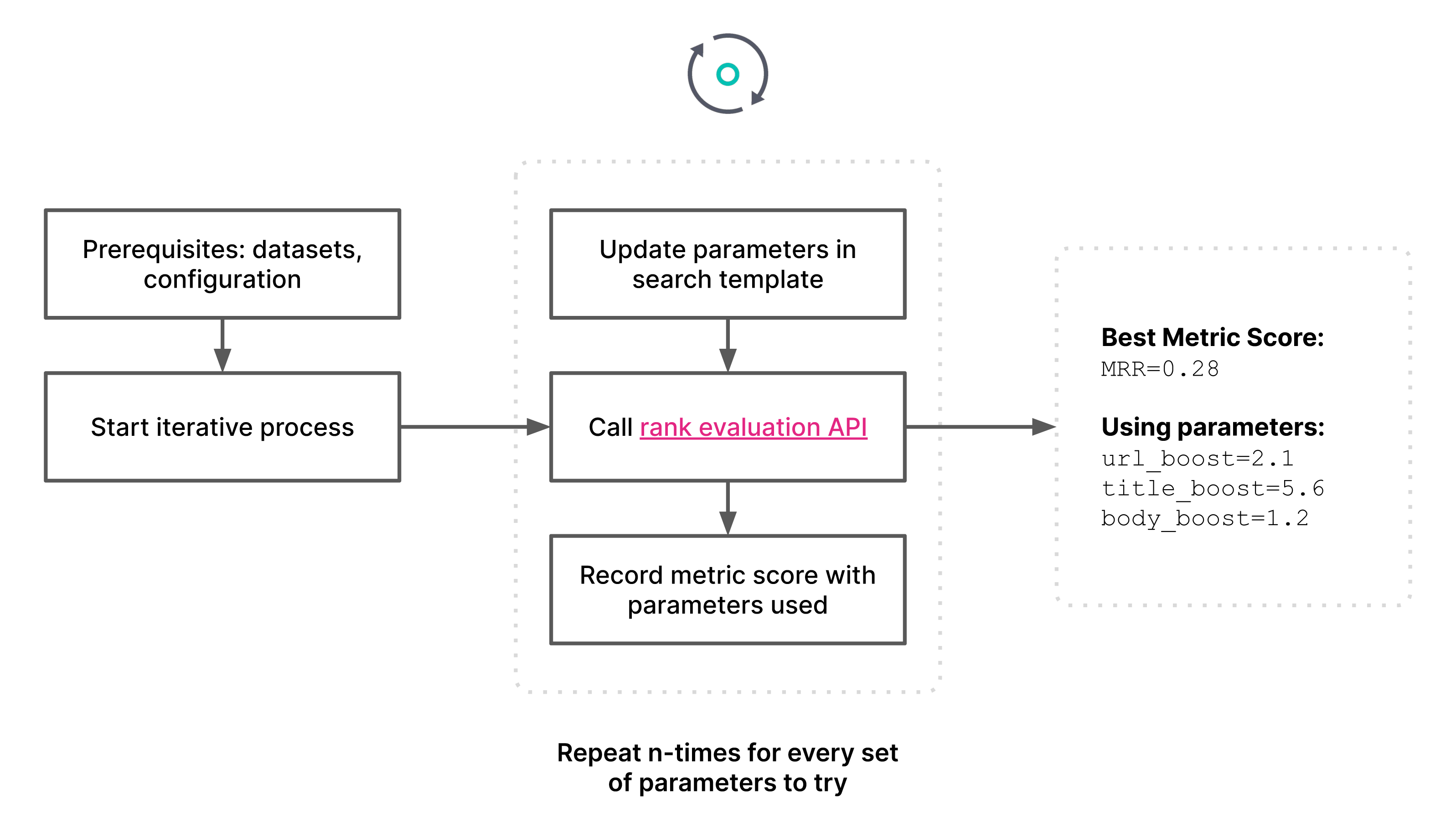
When we talk about parameters, such as url_boost, title_boost or body_boost from our example above, and the possible values that they can take on, we use the term parameter space. A parameter space is the world of possible values from all the parameters combined. In the context of parameter optimization (picking the parameter values that maximize some metric or score), we have the parameters plus the metric score. Let’s take a simple example of a parameter space of size two or a two-dimensional parameters space, with parameters x and y. Since we have just two dimensions, we can easily plot this parameter space in a 3D plot. In this case we use a contour plot where the third dimension, the color gradient, represents the metric score. The colour gradient goes from blue being the lowest metric score and yellow the highest (higher is better).
Grid search
To produce a plot like we saw above, we call the Rank Evaluation API with all possible permutations of the two parameters and store the returned metric score each time. In pseudo code it might look something like this:
for x in [1, 2, 3, 4, 5]:
    for y in [1, 2, 3, 4, 5]:
       params = {‘x’: x, ‘y’: y}
       score = rank_eval(search_template, relevance_data,
                         metric, params)
This double loop would then produce a table of metric scores:
    1  2  3  4  5
5:  0  5  7  3  0
4:  5  7  9  7  5
3:  0  7  9  10 4
2:  0  5  7  9  0
1:  0  2  6  5  2
A parameter space as in Figure 4 where x and y are a range of size 5 means that we call the Rank Evaluation API 25 (5*5) times. If we double the size of each parameter range to 10 we get a parameter space of size 100 (10*10). If we add to the number of parameters, say a z dimension, but keep the range the same, we get an even larger number of executions of the Rank Evaluation API — 125 (5*5*5).
When the parameter space is small, grid search is a good option because it’s exhaustive — it tests all possible combinations. However with the rapid and sometimes exponential growth in the number of calls to the Rank Evaluation API with a large parameter space, a grid search becomes impractical as it can increase the time needed to optimize a query to hours or even days. Remember that when calling the Rank Evaluation API, it will execute all queries in our dataset. That could be hundreds or thousands of queries that it needs to run on each call and for large corpora or complex search queries, that can be very time consuming even on a large Elasticsearch cluster.
Bayesian optimization
A more computationally efficient approach to parameter optimization is Bayesian optimization. Instead of trying all possible parameter value combinations as in a grid search, Bayesian optimization makes decisions about which parameter values to try next based on the previous metric scores. Bayesian optimization will look for areas of the parameter space that it hasn’t seen already but looks like it might contain better metric scores. Take the following parameter space as an example.

In Figure 5, we randomly placed ten black X marks. The red X marks the spot in the parameter space with the maximum metric score. Based on the random black X marks, we can already learn a little bit about the parameter space. The X marks in the bottom left and bottom right corners don’t look like very promising areas and it’s probably not worth testing more parameter values in that neighbourhood. If we look in the top portion of the parameter space, we can see a few points with much higher metric scores. We see particularly high values in the four X marks in the middle and this looks like a much more promising area in which to find our maximum metric score. Bayesian optimization will use these initial random points plus any subsequent points that it tries, and apply some statistics to pick the next parameter values to try. Statistics working hard for us — thank Bayes for that!
Results
Using the techniques outlined here and based on a series of evaluations with various analyzers, query types, and optimizations, we’ve made some improvements over baseline, un-optimized queries on the MS MARCO document ranking4 challenge. All experiments with full details and explanations can be found in the referenced Jupyter notebook, but below you can see the summary5 of our results. We see a progression from simple and un-optimized queries, and through parameter optimization, queries with higher MRR@100 scores (higher is better, the best scores from each notebook are highlighted in red). This shows us that we can indeed use data and a principled approach to improve search relevance by optimizing query parameters!
| Reference notebook | Experiment | MRR@100 |
| 0 - Analyzers | Default analyzers, combined per-field matches | 0.2403 |
| Custom analyzers, combined per-field matches | 0.2504 | |
| Default analyzers, multi_match cross_fields (default params) | 0.2475 | |
| Custom analyzers, multi_match cross_fields (default params) | 0.2683 | |
| Default analyzers, multi_match best_fields (default params) | 0.2714 | |
| Custom analyzers, multi_match best_fields (default params) | 0.2873 | |
| 1 - Query tuning | multi_match cross_fields baseline: default params | 0.2683 |
| multi_match cross_fields tuned (step-wise): tie_breaker, minimum_should_match | 0.2841 | |
| multi_match cross_fields tuned (step-wise): all params | 0.3007 | |
| multi_match cross_fields tuned (all-in-one v1): all params | 0.2945 | |
| multi_match cross_fields tuned (all-in-one v2, refined parameter space): all params | 0.2993 | |
| multi_match cross_fields tuned (all-in-one v3, random): all params | 0.2966 | |
| 2 - Query tuning - best_fields | multi_match best_fields baseline: default params | 0.2873 |
| multi_match best_fields tuned (all-in-one): all params | 0.3079 |
| Update (25 November 2020): Our official submission is in and we've achieved a score on the evaluation query set (only used for leaderboard rankings) of MRR@100 0.268. This gives us the best score for a non-neural (not using deep learning) ranker on the leaderboard! Stay tuned for more updates. Update (20 January 2021): We've improved on our first submission with the addition of a technique called doc2query (T5), as well as some other smaller fixes and improvements. With the new submission, we've achieved a score on the evaluation query set of MRR@100 0.300. That's a boost of +0.032 over our previous submission! More details can be found in the project README and accompanying Jupyter notebooks. |
Guidelines for success
We’ve seen now two approaches to optimizing queries and what kind of results we can achieve on the MS MARCO document ranking challenge. In order to help you be successful in optimizing your own queries, here are some tips and general guidelines to keep in mind.
- Since these approaches are data-driven, it’s very important that you have enough quality data. These approaches are only as good as your data is. “Enough” generally means at least hundreds of queries with labeled results. “Quality” means the data should be accurate and representative of the kinds of queries you are trying to improve and optimize.
- This is not a complete replacement for manual relevance tuning: debugging scores, building good analyzers, understanding your users and their information needs, etc.
- Bayesian optimization is sensitive to it’s own parameters. Observe how many total iterations you need, and how many random initializations to use to seed the process. If you have a large parameter space, you should consider a step-wise approach to break it up.
- Beware of overfitting with large parameter spaces. Think about cross validation to help correct for this but be aware that you would need to do this yourself in Python for now.
- Parameters will be tuned for a specific corpus and query set. They likely will not transfer unless the general statistics of the other corpus and query set are similar enough. This might also mean you need to re-tune on a regular basis in order to maintain the optimal parameters.
Conclusion
There’s a lot in this blog post and we hope that you’ve managed to follow along with us until now! The code examples and Jupyter notebooks show very concretely how to go through and tune a query. The principles are not limited to query parameters, so there’s also an example notebook showing how to tune BM25 parameters. We hope you get a chance to check out those examples and do some experimentation of your own. We’ve had the most success using isolated, large-scale Elastic Cloud clusters that we spin up and shutdown whenever we need them. Now go forth, and use your own data to optimize your queries! Don’t forget to bring your questions or success stories to our discussion forums.
Sources
1 Click Models for Web Search by Aleksandr Chuklin, Ilya Markov and Maarten de Rijke
2 Conversion Models: Building Learning to Rank Training Data by Doug Turnbull
3 A Dynamic Bayesian Network Click Model for Web Search Rankingby Olivier Chapelle
4 We rank all documents in a single ranking phase, then take the top 100 for MRR. This is considered a "full ranking" approach, as opposed to "re-ranking" which only tries to re-rank the top 1,000 candidate documents from a pre-set list of results.
5 These results are current as of the publication date of this post, but the project README will contain up-to-date results if we continue to experiment with new techniques.