How to map custom boundaries in Kibana with reverse geocoding
Want to create a map of where your users are? With the GeoIP processor, you can easily attach the location of your users to your user metrics.
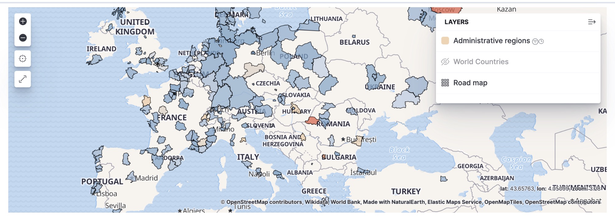
Right out of the box, Kibana can map this traffic immediately by country or country subdivision:
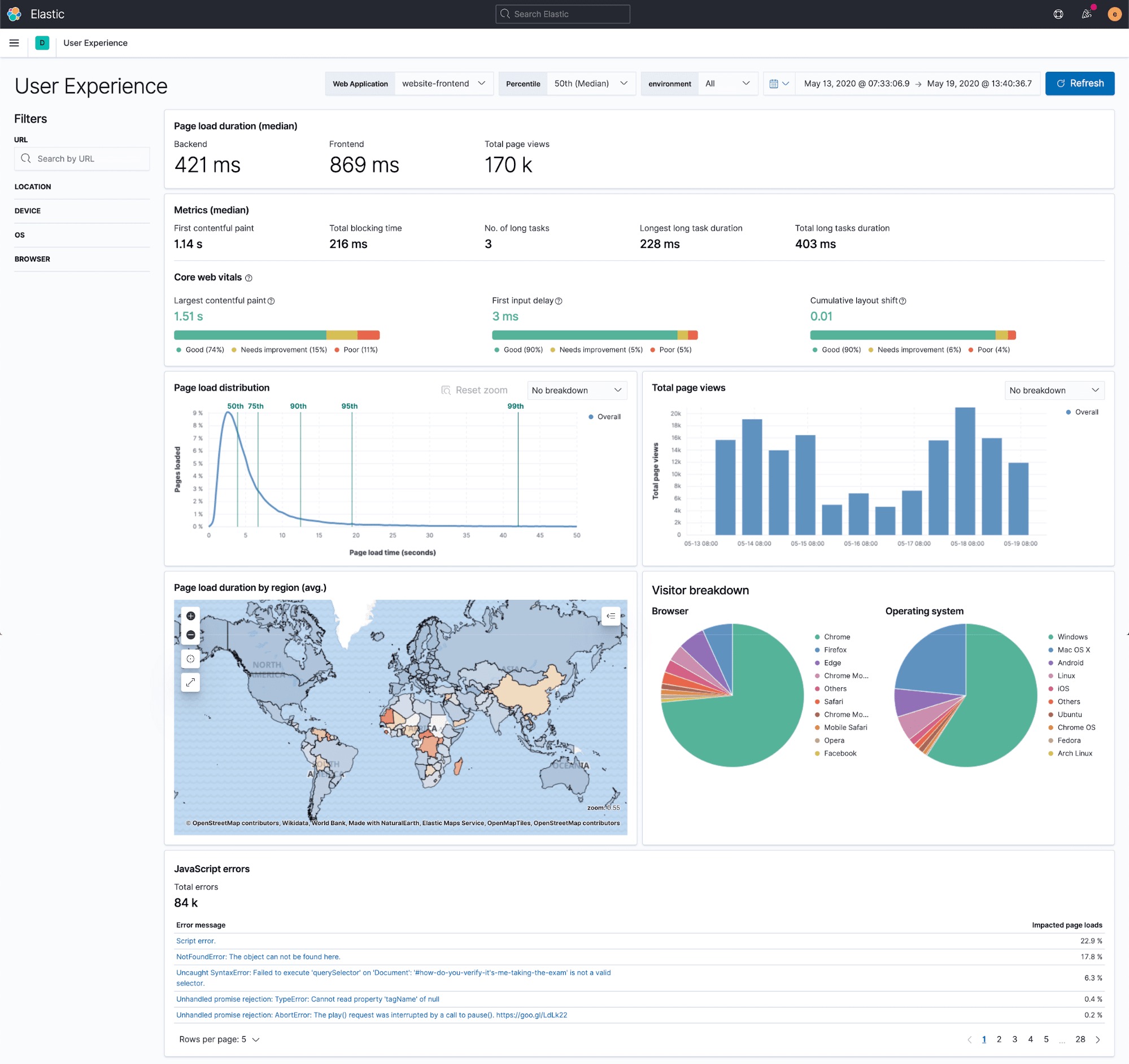
Plus, the new User Experience app for Elastic APM automatically creates maps based on monitoring data:
But what if you want to take this one step further and create maps with different regions?
Custom regions: metro area, proximity to IKEA, anything...
Elastic Maps come with a lot of great region options so you can get started quickly, but it also offers the ability to easily map your own regions. You can use any boundary data you'd like for this, as long as you have source data that contains a longitude and latitude.
For this example, suppose we use GeoIP, which is built into Elasticsearch. GeoIP is a common way of transforming an IP address to a longitude and latitude.
GeoIP is roughly accurate on the city level globally and neighborhood level in selected countries. It’s not as great as an actual GPS location from your phone, but it’s much more precise than just a country, state, or province. So there’s a lot of resolution between the precision of the longitude and latitude from GeoIP and the default maps you get in Kibana.
This level of detail can be very useful for driving decision-making. For example, say you want to spin up a marketing campaign based on the locations of your users or show executive stakeholders which metro areas you see are experiencing an uptick of traffic.
That kind of scale in the United States is often captured with what the Census Bureau calls the Combined Statistical Area (CSA). It is roughly equivalent with how people intuitively think of which urban area they live in. It does not necessarily coincide with state or city boundaries.
This subdivision is central to many of the Federal Government’s policies, such as making cost-of-living adjustments to fiscal benefits. CSAs generally share the same telecom providers and ad networks. New fast food franchises expand to a CSA rather than a particular city or municipality. Basically, people in the same CSA shop in the same IKEA.
Assigning a spatial identifier to a feature based on its location is called reverse geocoding or spatial joining. It’s one of the most common operations in geographic information systems (GIS).
In the Elastic Stack, this reverse-geocoding functionality resides within Elasticsearch via the enrich processor. Here we're going to use Kibana to manage these processors and then create maps and visualizations. In the tutorial below, we will use CSA boundaries to illustrate reverse geocoding.
Reverse geocoding with the Elastic Stack
Step 1: Indexing the geospatial data
This will probably be the most custom part of any solution, so we’ll skip it 😜. Most integrations can rely on the GeoIP processor to transform an IP location into a geo_point field.
Whatever process you have used to index your data, you’ll have a document using the ECS schema that will contain two sets of fields created by the GeoIP processor:
- destination.geo.* for where requests are going (usually a data center)
- client.geo.* for the origin of the request, sometimes called
origin.geo.*.
The relevant bit here is that *.geo.location field. It contains the longitude and latitude of the device.
For the rest of this tutorial, we’ll use the kibana_sample_data_logs index that comes with Kibana, since that’s quicker to follow along with. The critical part for reverse geocoding is the presence of the longitude/latitude information and less how that longitude/latitude field was created.
Step 2: Indexing the boundaries
To get the CSA boundary data, download the Cartographic Boundary shapefile (.shp) from the Census Bureau’s website.
To use it in Kibana, we need it as a GeoJSON format. I used QGIS to convert it to GeoJSON. Check out this helpful tutorial if you'd like to do the same.
Once you have your GeoJSON file, go to Maps in Kibana and upload the data using the GeoJSON uploader.
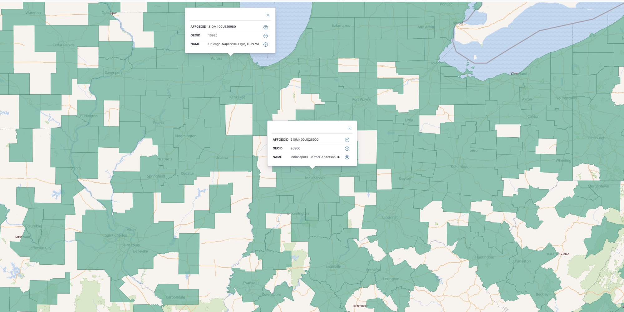
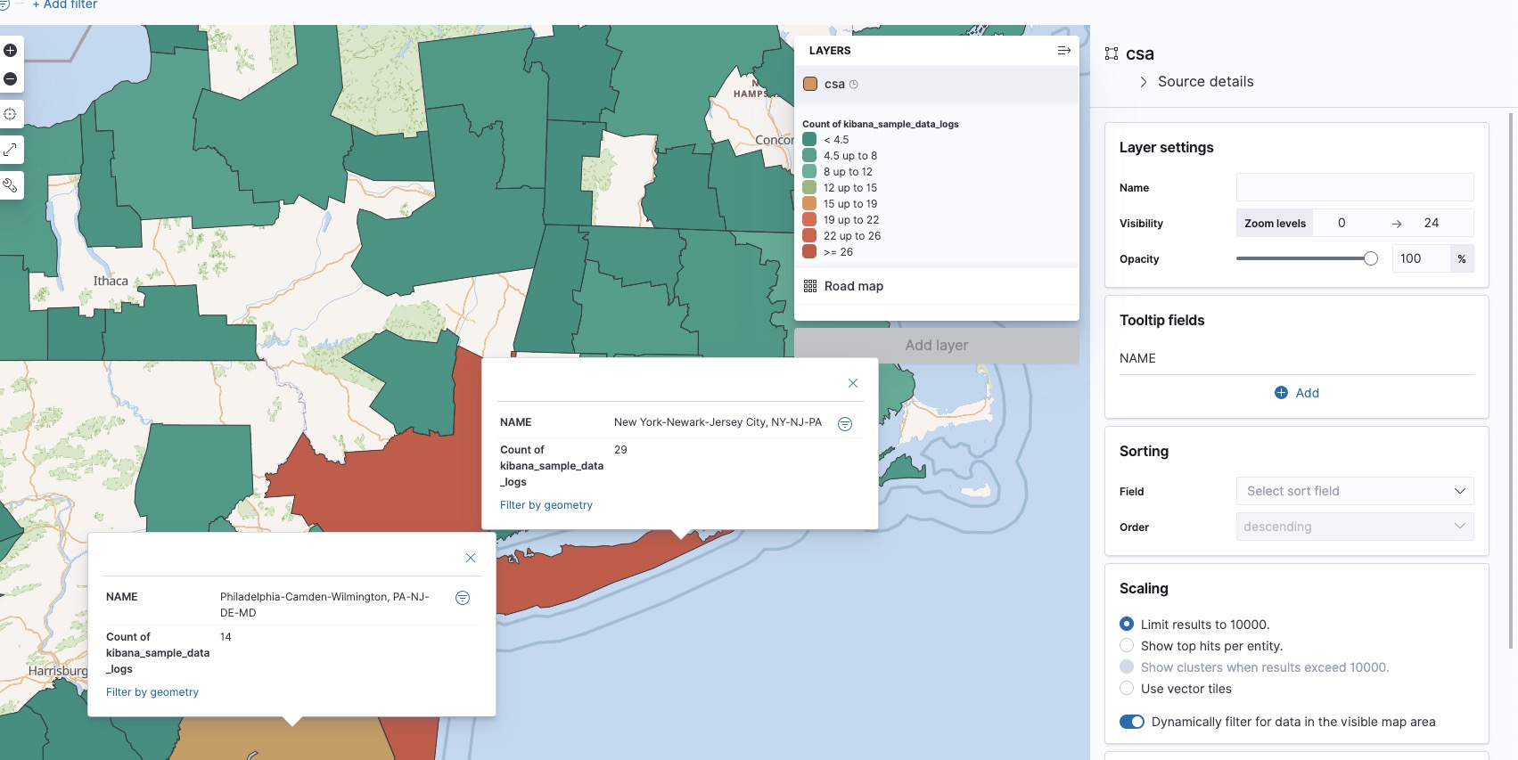
Zoomed in on the result, we get a sense of what exactly constitutes a metro area in the eyes of the Census Bureau. I added some tooltip fields using the Tooltip Fields in the layer editor.
This upload created our CSA index containing the shapes we’ll use for reverse geocoding.
Step 3: Reverse geocoding with a pipeline
In order to create our pipeline, we first need to create the reverse geocoder. We can do this by creating a geo_match enrichment policy.
Run the following from Dev Tools in Kibana:
PUT /_enrich/policy/csa_lookup
{
  "geo_match": {
    "indices": "csa",
    "match_field": "coordinates",
    "enrich_fields": [ "GEOID", "NAME"]
  }
}
POST /_enrich/policy/csa_lookup/_execute
This creates an enrich policy called csa_lookup. It uses the coordinates field which contains the shapes (it has a geo_shape field-type). The policy will enrich other documents with the GEOID and NAME fields. It also automatically attaches the coordinates field. The _execute call is required for initializing the policy.
Then we’ll integrate this reverse-geocoder into a pipeline.
PUT _ingest/pipeline/lonlat-to-csa
{
  "description": "Reverse geocode longitude-latitude to combined statistical area",
  "processors": [
    {
      "enrich": {
        "field": "geo.coordinates",
        "policy_name": "csa_lookup",
        "target_field": "csa",
        "ignore_missing": true,
        "ignore_failure": true,
        "description": "Lookup the csa identifier"
      }
    },
    {
      "remove": {
        "field": "csa.coordinates",
        "ignore_missing": true,
        "ignore_failure": true,
        "description": "Remove the shape field"
      }
    }
  ]
}
Our pipeline consists of two processors:
- The first is the
enrichprocessor we just created. It references ourcsa_lookuppolicy. It creates a new fieldcsathat contains the CSA identifiers (GEOID, NAME) and the CSA geometry (coordinates). - The second is a
removeprocessor that removes the CSA geometry field. (We don’t need it since we are only interested in the identifiers).
Step 4: Running the pipeline on all your documents
Now that the pipeline is created, we can start using it. And a great thing about pipelines is you can run them on your existing data.
With _reindex, you can create a new index with a copy of your newly enriched documents:
POST _reindex
{
  "source": {
    "index": "kibana_sample_data_logs"
  },
  "dest": {
    "index": "dest",
    "pipeline": "lonlat-to-csa"
  }
}
With _update_by_query, all the documents are enriched in place:
POST kibana_sample_data_logs/_update_by_query?pipeline=lonlat-to-csa
Step 5: Running the pipeline on new documents at ingest
All the existing docs are updated. Now we need to make sure we also use this pipeline when indexing new documents:
POST kibana_sample_data_logs/_doc/testdoc?pipeline=lonlat-to-csa
{
  "geo": {
    "coordinates": {
      "lon": -85.7585,
      "lat": 38.2527
    }
  }
}
Let's test it out:
GET kibana_sample_data_logs/_doc/testdoc
You can also setup a default pipeline to have this reverse geocoding done for each incoming document by default:
PUT kibana_sample_data_logs/_settings
{
  "index": {
    "default_pipeline": "lonlat-to-csa"
  }
}
Step 6: Creating a map
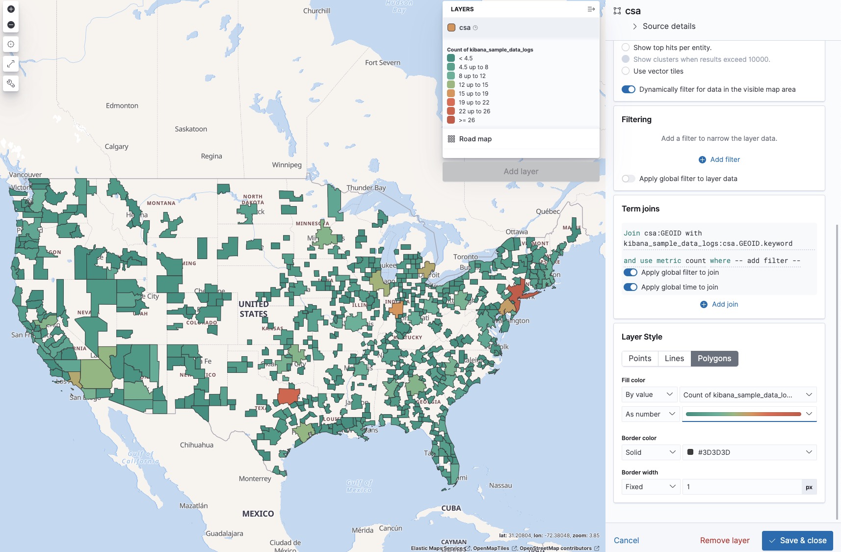
Back in the Maps app, click Add layer. Then select Choropleth Layer:
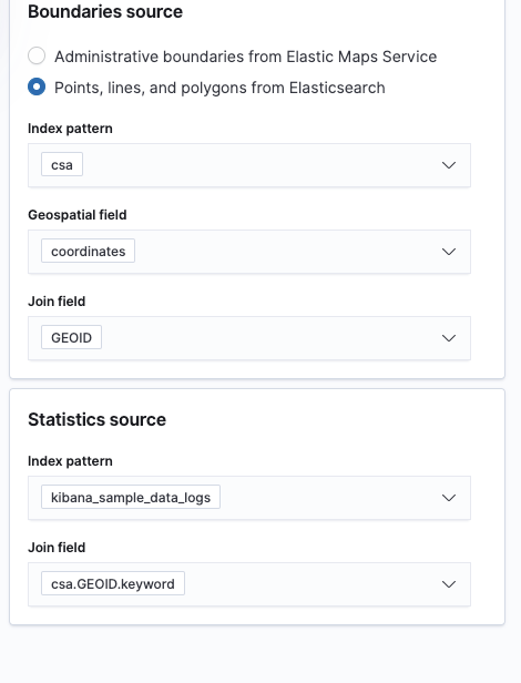
We’ll select our CSA -layer (these are the shapes), and join them by the unique GEOID identifier. Then we’ll join the aggregate info from our request index. The join field here is csa.GEOID, which was created by the pipeline.
After changing the default color ramp from green to red and adding some tooltip fields, we can now create our map. In this case, it shows a few hotspots in the Dallas, Indianapolis, and New York metropolitan areas.
Get started today
Hopefully this got you thinking about how to use a reverse geocoder. It’s an incredibly powerful tool to create custom maps and gain new insights in your data. If you're not already using Elastic Maps, try it out free in Elastic Cloud.
For any feedback and questions, our Discuss forums are the perfect venue. And if you find yourself breaking the boundaries (ha!) of your old mapping limitations, show us what you made! Connect with us in the forums or @ us on Twitter.