Hexagonal spatial analytics in Elasticsearch

Elasticsearch 8.7.0 can do some very cool geo-spatial aggregations over a hexagonal grid, which has nice advantages over the existing rectangular grid we’ve been using for years. This feature has been introduced over the last few releases and is now really worth bragging about.

How did we get there? In 2018 Uber announced it had open sourced the H3 library, enabling hexagonal tiling of the planet for much better analytics of the company’s traffic and regional pricing models.

In late 2021, we evaluated the option of porting the Uber H3 library from C to Java for possible inclusion in Elasticsearch. This project went very well, and in early 2022 was released as a standalone artifact under the Apache2 license, as well as part of a new hexagonal aggregation feature within Elasticsearch and Kibana 8.1. While that was a fantastic addition to Elasticsearch, it did have one very clear limitation: aggregations only worked on point data, specifically fields mapped as geo_point. Now in Elasticsearch 8.7, we are pleased to announce support for geo_shape aggregations as well as many performance and memory improvements to our port of H3.

Boosting H3 on Java

First, let’s talk about how we improved our version of the H3 library. The original port aimed to be a faithful copy of the Uber C code, translated into Java. This worked well enough for the earlier release of hexagonal aggregations over geo_point data, but as we enhanced this to support the much more complex problem of aggregating geo_shape data, we realized the performance of the library needed to improve. 

We developed microbenchmarks in order to compare the performance of the java bindings provided by Uber’s H3 library with our Java implementation and we noticed that two functions were significantly slower: the method that resolves a latitude/longitude pair into an H3 cell and the function that returns the boundary of an H3 cell:

When investigating these differences, we discovered that there were many parts of the library that needed to be optimized for both memory and performance:

• We refactored the code to be more in line with Java standards and worked to minimize the object allocation since these functions will be called in hot loops.
• We used a faster trigonometric math implementation based on the fdlibm package.
• We used planar 3d math whenever possible to try to minimize the number of calls to trigonometric functions.

After these changes, the performance improvements were very satisfactory:

In addition to this, our needs were not always supported by existing functions in the H3 library, and so additional functions were written. For example, we added a function that given an H3 cell, it returns the H3 cells at the child level that intersect the provided cell but are not part of the children set. This allowed us to optimize hexagonal aggregations geometrically.

Elasticsearch geohex aggregations

Elasticsearch originally introduced a geohash based grid aggregation over geo_point data way back in 2014. Over the years, this has been enhanced in several ways: first, the addition of `z/x/y` tiling as a superior mechanism to geohash, and second, the introduction of geo_shape as a supported field type for geo-grid aggregations.

Then in Elasticsearch 8.1, we added support for geo-grid tiling using H3 hexagonal grids over geo_point, and now finally in Elasticsearch 8.7 we’ve extended this support to geo_shape.

This development was challenging due to the different properties of the H3 grid in comparison to geotile or geohash grids. Geohash and geotile hierarchy has the property of geometric containment, which means that the children of a cell are fully contained by the cell. On the other hand, the Uber H3 hierarchy is only logical and the children of a cell are not fully contained, which makes navigating the hierarchy much more complicated.

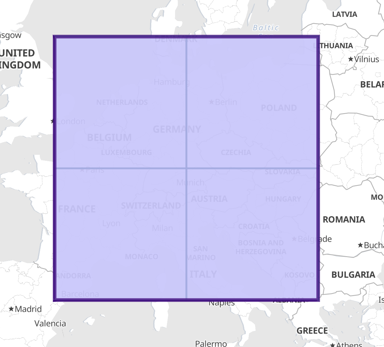
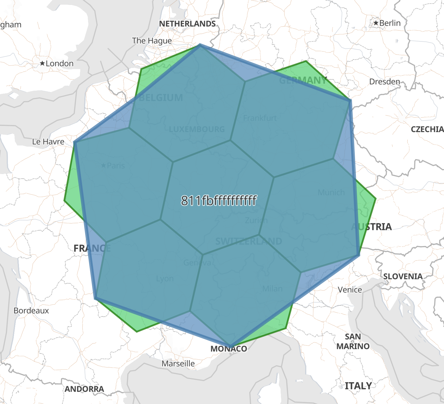
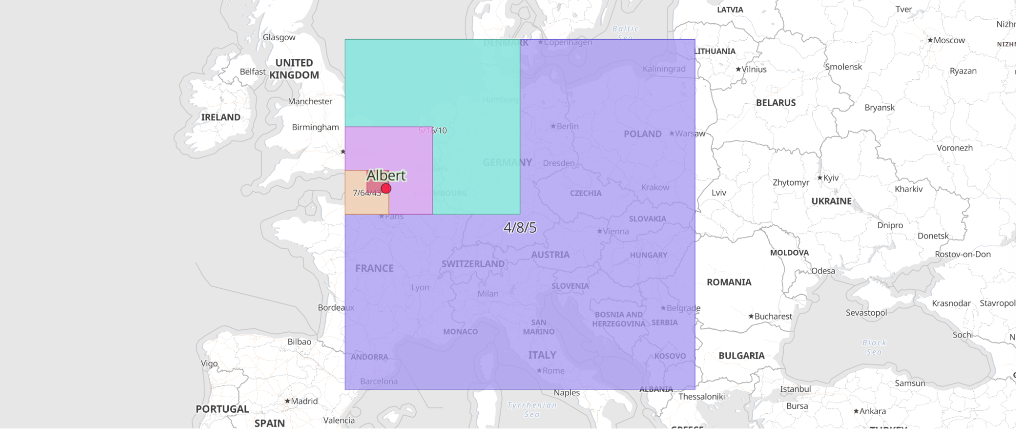
When performing aggregations over the grid at a specific resolution, what is done internally is to answer the question “which tiles at this resolution intersect a particular geometry?” With the geometric containment we see above, this can be implemented as a simple recursive algorithm: start at resolution 0, and if the tile intersects the geometry, recurse to the four child tiles (or 32 child tiles for geohash), and repeat the test. No child will be checked if its parent does not intersect, reducing the search space. Consider a search for the geotile containing the French city of “Albert” at precision 8. The following visualization shows the five steps from precision 4 to 8 of the search:

For geohex aggregations, however, we need to be a lot cleverer. In order to navigate the hierarchy geometrically, we added a new function to the H3 API, which returns the cells that are not logical children of a cell but still intersect the cell. Then we will navigate those cells if we detect that their parent cells are not part of the solution.

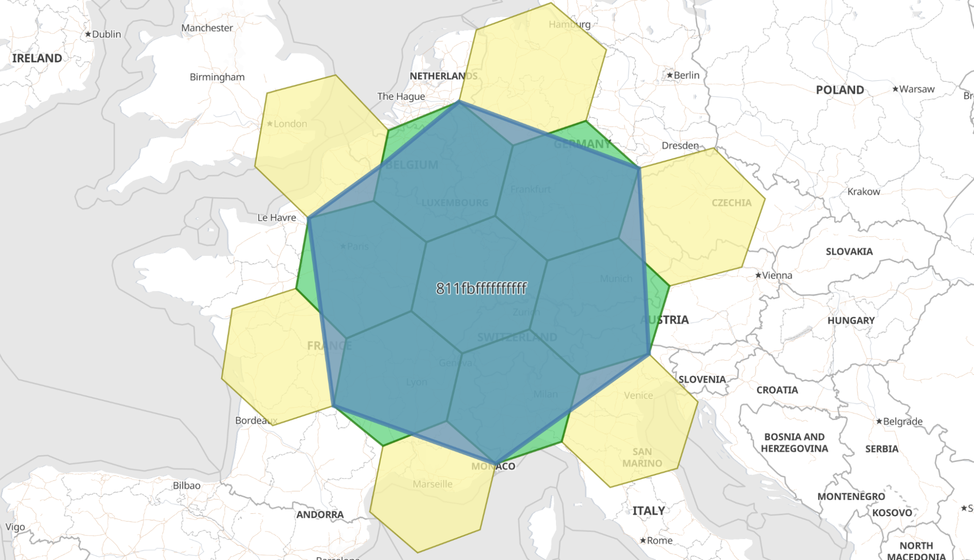
As with geotile and geohash aggregations, it is possible to traverse the hierarchy in a recursive way when asking the question “which tiles at this resolution intersect a particular geometry?” But we need to handle the case when a geometry intersects a child tile but not the parent tile (the light green parts in the image above), or conversely when a geometry intersects a parent tile, but not one of its children. These are the same concern and can be solved by using two recursion conditions evaluated at each parent cell:

• Search the direct children if the parent intersects (same condition as with geotile and geohex). This will cover the area of the child cells that intersect the parent cell.
• Also search the intersecting non-children (yellow cells in the image above) if the parent of those non-children does not intersect the geometry. This means we will only recurse down for the area of overlap between the yellow and blue above, and it completes the entire area covered by the parent cell.

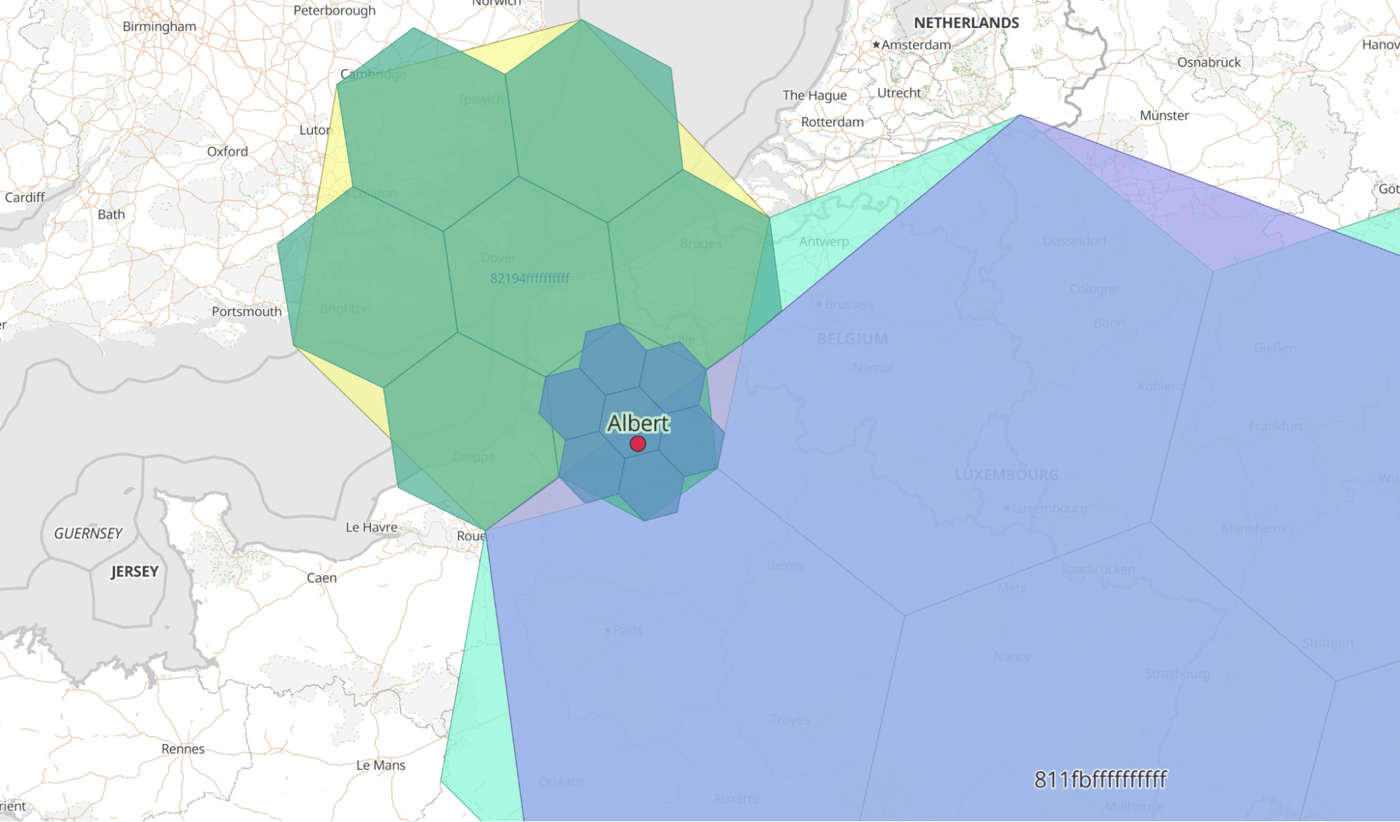
To clarify this, consider again a search for the town of “Albert” in France, where we can see that this town’s location intersects the cell “811fb” but not any of its children:

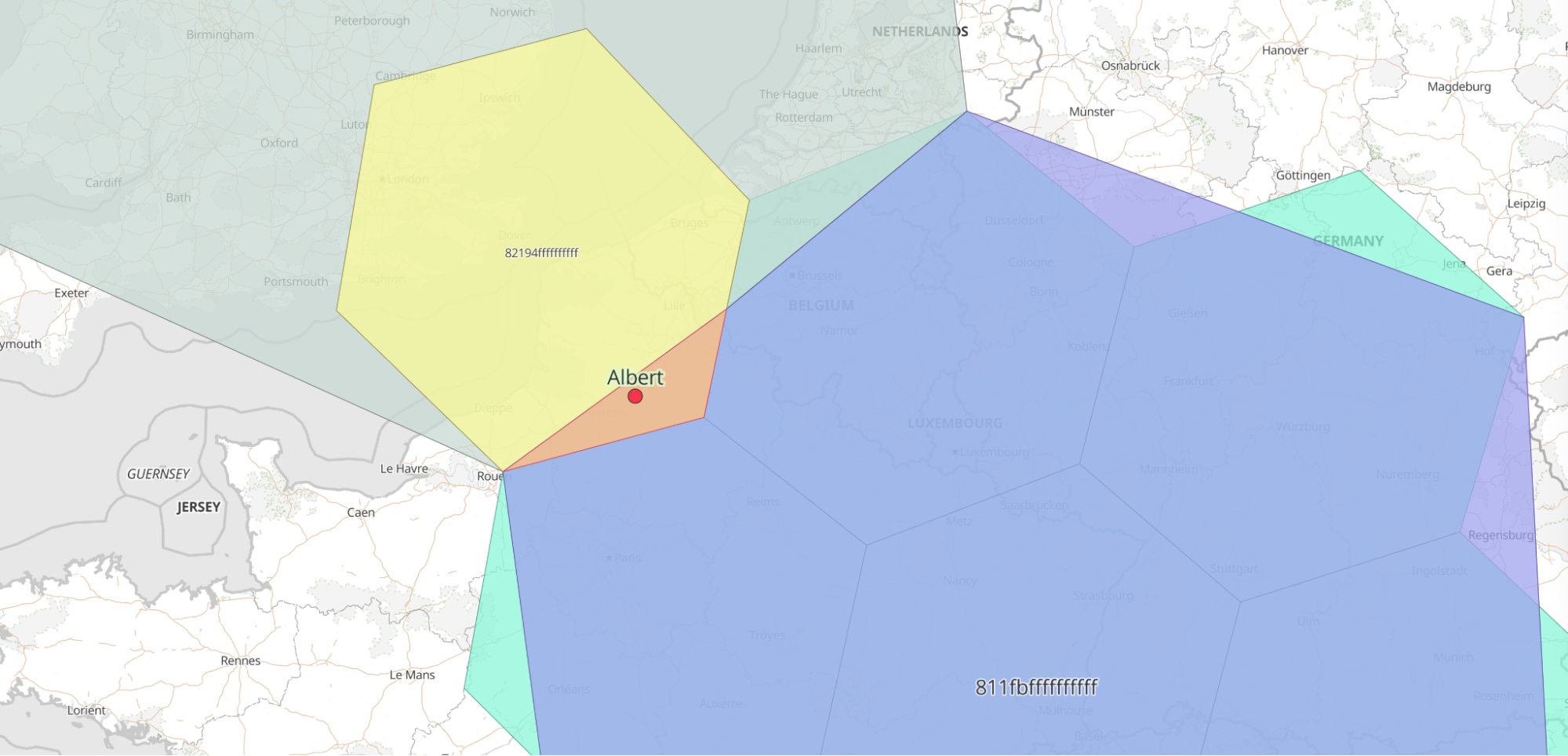
Repeatedly recursing down through either the intersecting children or the intersecting non-children will uniquely reach the cell that contains the point at the desired precision:

Kibana and geohex

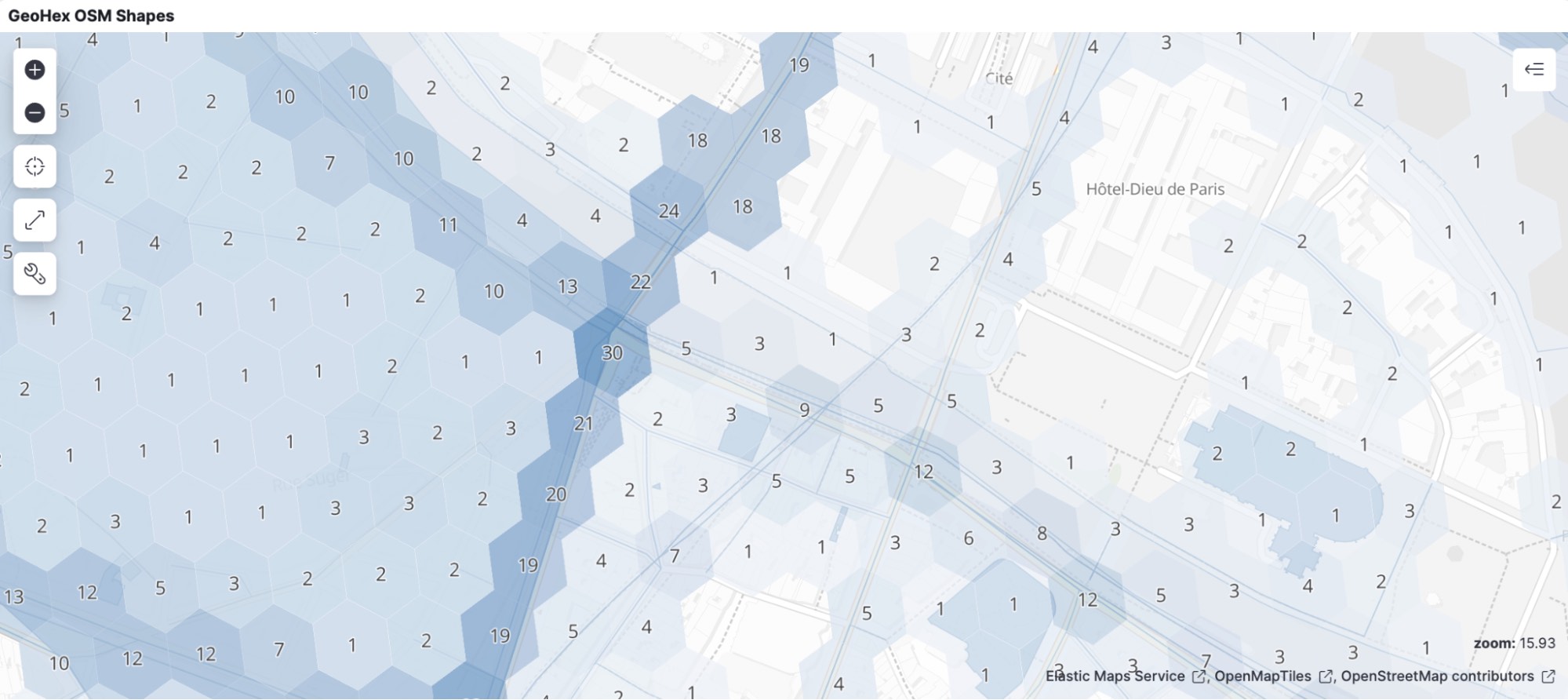
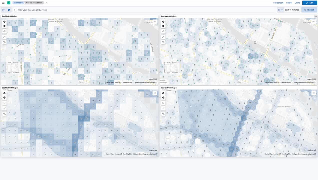
Kibana announced support for geohex aggregations over geo_point for version 8.1 in March 2022. Now in version 8.7, we support geohex aggregations over geo_shape as well. Let’s take a look at how to access this feature in Kibana maps.

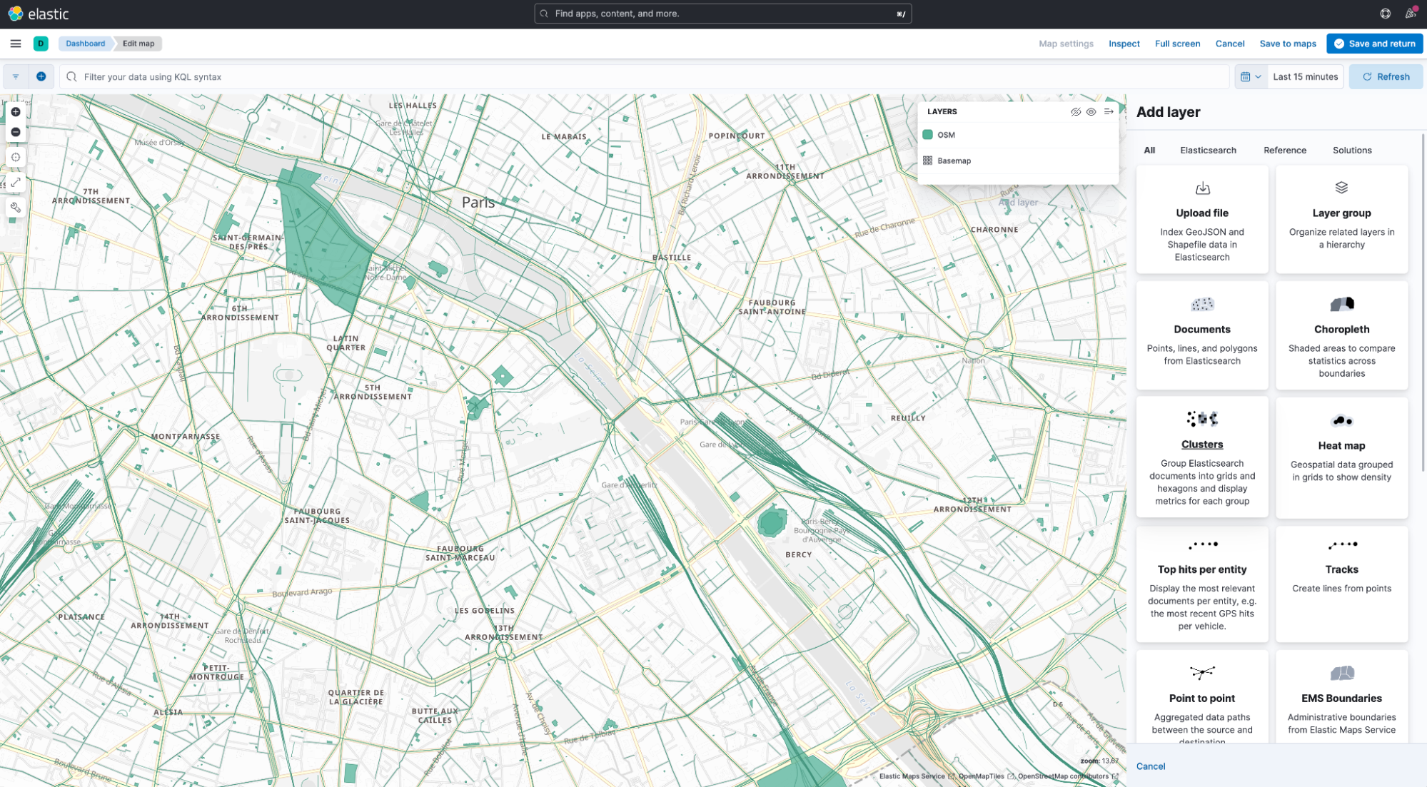
Assuming you have already loaded some spatial data containing geo_shape fields, it is possible to visualize the shapes themselves on the map by adding a Documents layer, as seen in the above screenshot. It is also possible to add a layer with the results of a tiled aggregation. This is achieved using the Clusters layer type, seen in the third row of layer types above.

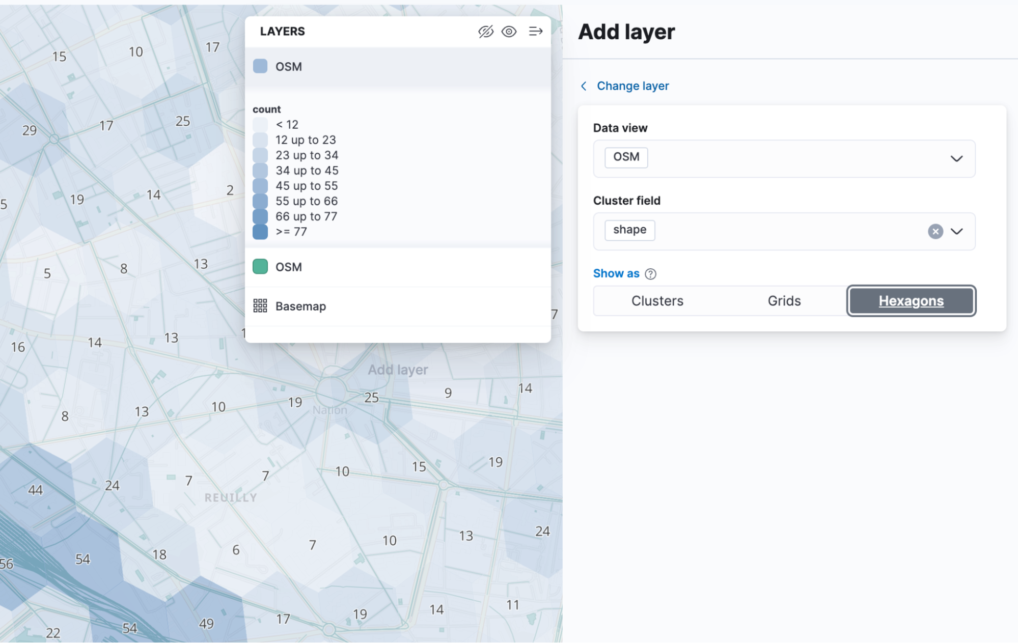
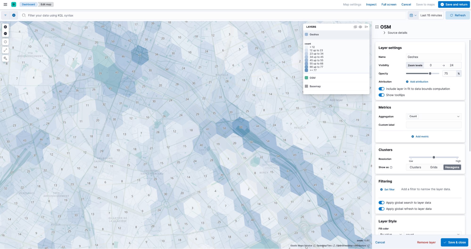
After selecting the data view and geo_shape field name you need to choose the geo-grid aggregation type. By default, Kibana selects Clusters, which will use a rectangular tiling but display as circles sized to the document count. You should select Grids for a geotile aggregation or Hexagons for a geohex aggregation. Finally click Add Layer, choose a layer name, and save the layer.

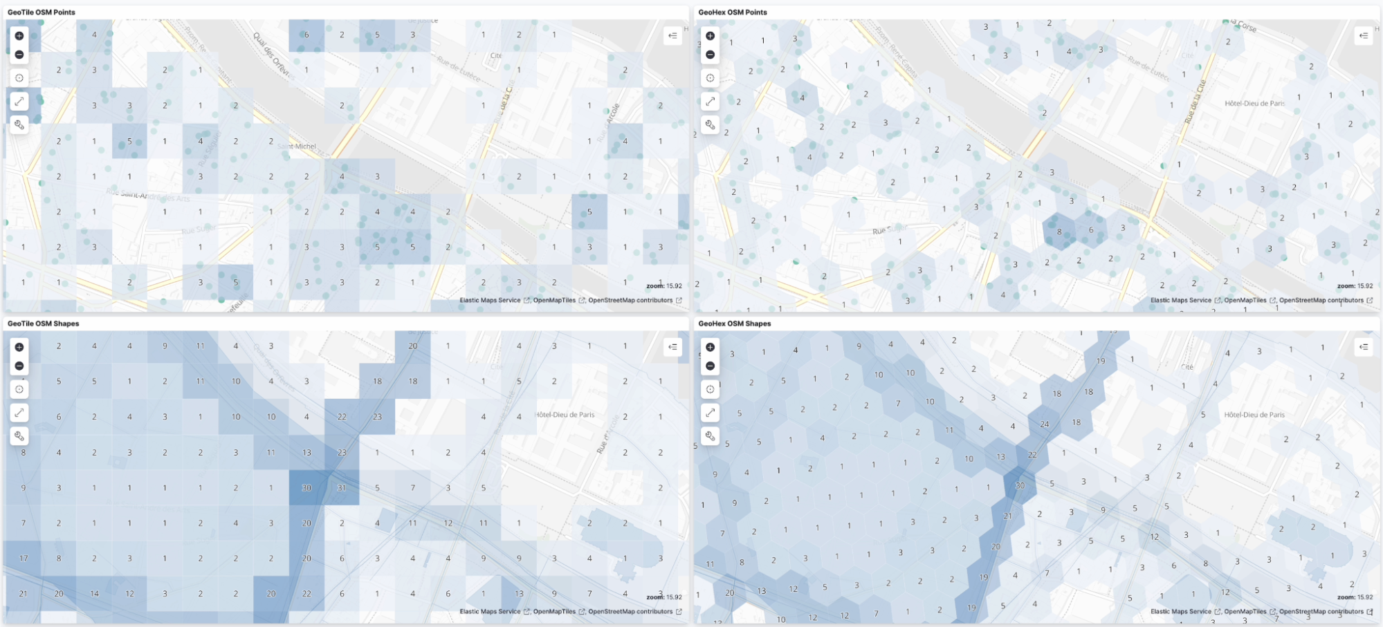
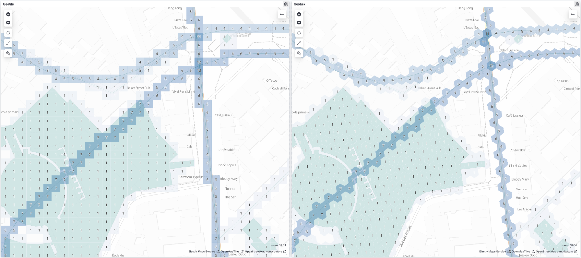
A very useful feature added to Kibana maps recently is the ability to synchronize the panning and zooming of two map views within the same dashboard. This allows us to compare and contrast different aggregations visually. Particularly relevant to the new geohex aggregation is the ability to contrast it with the already existing geotile aggregation. Or in terms of the Kibana UI, this means to add two cluster layers with Grid and Hexagon selected respectively.

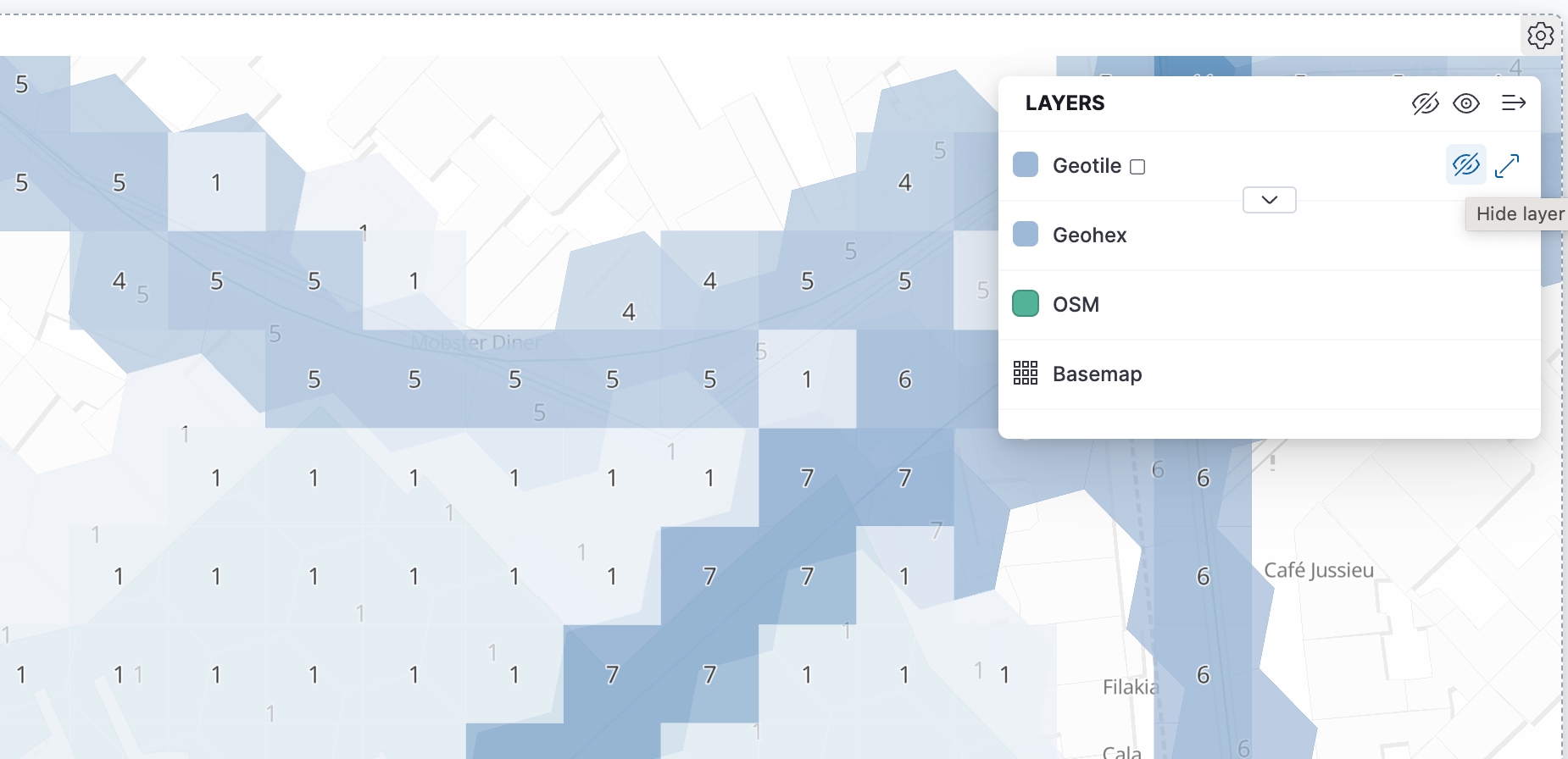
This can be achieved either by starting with a blank dashboard, and adding two maps to it, each with the relevant aggregation added, or by starting by creating a new map and adding it to an existing dashboard. One approach that is particularly flexible is to create a single map with both layers, add it to a dashboard, and then clone the map. In each copy, hide the layer you do not want to see with the hide layer icon.

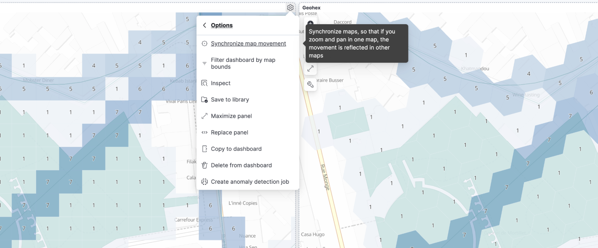
Finally, use the synchronize map movement option to synchronize the maps.

The result can be very striking in a demo.

To see this in action, take a look at this short video that demonstrates this new feature and compares it with the geotile grid aggregation over both geo_point and geo_shape.

Conclusions

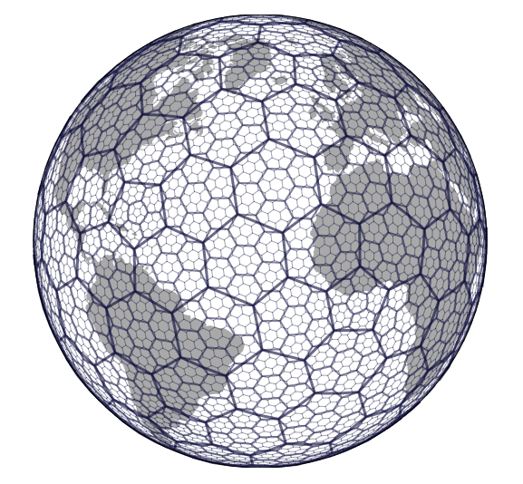
Geo-grid aggregations have been a useful feature of Elasticsearch and Kibana maps for a long time. The addition of hexagonal grids over the past few releases adds the power of the popular Uber H3 tiling approach to Elasticsearch aggregations and to Kibana cluster layers. This aggregation mechanism has many advantages over rectangular tiles, in particular the fact that the area of each tile is approximately the same all over the planet, allowing for far more relevant statistical results when compared to equi-rectangular grids, which have extreme distortions away from the equator. Also, the distance between each hexagonal tile and its neighbors is the same in all directions, which is not true for rectangular grids.

We hope you find this feature as useful as we do, and we welcome any feedback from users.

Do you want to learn more? Take a look at our reference documentation, or watch a video demo:

• Feature announcement: Geohex aggregations on both geo_point and geo_shape fields
• Reference documentation: Geohex grid aggregation
• Reference documentation: Aggregating geo_shape fields
• Video: Comparing geotile and geohex in Kibana
• Video: How geometric search works for hexagons
• Video: Creating a kibana demo of hexagonal clusters