Practical BM25 — Part 2: The BM25 Algorithm and its variables
This is the second post in the three-part Practical BM25 series about similarity ranking (relevancy). If you're just joining, check out Part 1: How Shards Affect Relevance Scoring in Elasticsearch.
The BM25 model
I’ll try to dive into the mathematics here only as much as is absolutely necessary to explain what’s happening, but this is the part where we look at the structure of the BM25 formula to get some insights into what’s happening. First we’ll look at the formula, then I’ll break down each component into understandable pieces:

We can see a few common components like qi, IDF(qi), f(qi,D), k1, b, and something about field lengths. Here’s what each of these is all about:
- qi is the ith query term.
For example, if I search for “shane,” there’s only 1 query term, so q0 is “shane”. If I search for “shane connelly” in English, Elasticsearch will see the whitespace and tokenize this as 2 terms: q0 will be “shane” and q1 will be “connelly”. These query terms are plugged into the other bits of the equation and all of it is summed up. - IDF(gi) is the inverse document frequency of the ith query term.
For those that have worked with TF/IDF before, the concept of IDF may be familiar to you. If not, no worries! (And if so, note there is a difference between the IDF formula in TF/IDF and IDF in BM25.) The IDF component of our formula measures how often a term occurs in all of the documents and “penalizes” terms that are common. The actual formula Lucene/BM25 uses for this part is:
Where docCount is the total number of documents that have a value for the field in the shard (across shards, if you’re using search_type=dfs_query_then_fetch) and f(qi) is the number of documents which contain the ith query term. We can see in our example that “shane” occurs in all 4 documents so for the term “shane” we end up with an IDF(“shane”) of:
However, we can see that “connelly” only shows up in 2 documents, so we get an IDF(“connelly”) of:
We can see here that queries containing these rarer terms (“connelly” being rarer than “shane” in our 4-document corpus) have a higher multiplier, so they contribute more to the final score. This makes intuitive sense: the term “the” is likely to occur in nearly every English document, so when a user searches for something like “the elephant,” “elephant” is probably more important — and we want it to contribute more to the score — than the term “the” (which will be in nearly all documents). - We see that the length of the field is divided by the average field length in the denominator as fieldLen/avgFieldLen.
We can think of this as how long a document is relative to the average document length. If a document is longer than average, the denominator gets bigger (decreasing the score) and if it’s shorter than average, the denominator gets smaller (increasing the score). Note that the implementation of field length in Elasticsearch is based on number of terms (vs something else like character length). This is exactly as described in the original BM25 paper, though we do have a special flag (discount_overlaps) to handle synonyms specially if you so desire. The way to think about this is that the more terms in the document — at least ones not matching the query — the lower the score for the document. Again, this makes intuitive sense: if a document is 300 pages long and mentions my name once, it’s less likely to have as much to do with me as a short tweet which mentions me once. - We see a variable b which shows up in the denominator and that it’s multiplied by the ratio of the field length we just discussed. If b is bigger, the effects of the length of the document compared to the average length are more amplified. To see this, you can imagine if you set b to 0, the effect of the length ratio would be completely nullified and the length of the document would have no bearing on the score. By default, b has a value of 0.75 in Elasticsearch.
- Finally, we see two components of the score which show up in both the numerator and the denominator: k1 and f(qi,D). Their appearance on both sides makes it hard to see what they do by just looking at the formula, but let’s jump in quickly.
- f(qi,D) is “how many times does the ith query term occur in document D?” In all of these documents, f(“shane”,D) is 1, but f(“connelly”,D) varies: it’s 1 for documents 3 and 4, but 0 for documents 1 and 2. If there were a 5 th document which had the text “shane shane,” it would have f(“shane”,D) of 2. We can see that f(qi,D) is in both the numerator and the denominator, and there’s that special “k1” factor which we’ll get to next. The way to think about f(qi,D) is that the more times the query term(s) occur a document, the higher its score will be. This makes intuitive sense: a document that has our name in it lots of time is more likely to be related to us than a document that has it only once.
- k1 is a variable which helps determine term frequency saturation characteristics. That is, it limits how much a single query term can affect the score of a given document. It does this through approaching an asymptote. You can see the comparison of BM25 against TF/IDF in this:
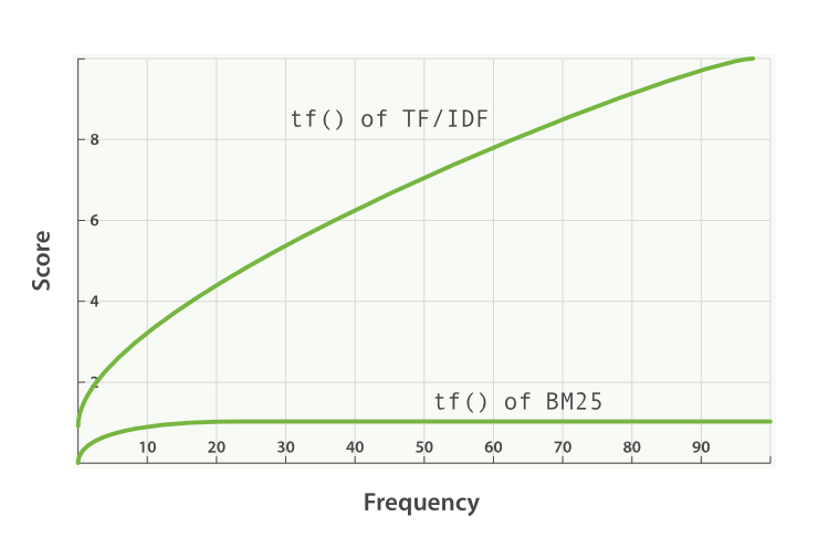
A higher/lower k1 value means that the slope of “tf() of BM25” curve changes. This has the effect of changing how “terms occurring extra times add extra score.” An interpretation of k1 is that for documents of the average length, it is the value of the term frequency that gives a score of half the maximum score for the considered term. The curve of the impact of tf on the score grows quickly when tf() ≤ k1 and slower and slower when tf() > k1.
Continuing with our example, with k1 we’re controlling the answer to the question “how much more should adding a second ‘shane’ to the document contribute to the score than the first or the third compared to the second?” A higher k1 means that the score for each term can continue to go up by relatively more for more instances of that term. A value of 0 for k1 would mean that everything except IDF(qi) would cancel out. By default, k1 has a value of 1.2 in Elasticsearch.
Revisiting our search with our new knowledge
We’ll delete our people index and recreate it with just 1 shard so that we don’t have to use search_type=dfs_query_then_fetch. We’ll test our knowledge by setting up three indices: one with the value of k1 to 0 and b to 0.5 and a second index (people2) with the value of b to 0 and of k1 to 10 and a third index (people3) with a value of b to 1 and k1 to 5.
DELETE people
PUT people
{
  "settings": {
    "number_of_shards": 1,
    "index" : {
        "similarity" : {
          "default" : {
            "type" : "BM25",
            "b": 0.5,
            "k1": 0
          }
        }
    }
  }
}
PUT people2
{
  "settings": {
    "number_of_shards": 1,
    "index" : {
        "similarity" : {
          "default" : {
            "type" : "BM25",
            "b": 0,
            "k1": 10
          }
        }
    }
  }
}
PUT people3
{
  "settings": {
    "number_of_shards": 1,
    "index" : {
        "similarity" : {
          "default" : {
            "type" : "BM25",
            "b": 1,
            "k1": 5
          }
        }
    }
  }
}
Now we’ll add a few documents to all three indices:
POST people/_doc/_bulk
{ "index": { "_id": "1" } }
{ "title": "Shane" }
{ "index": { "_id": "2" } }
{ "title": "Shane C" }
{ "index": { "_id": "3" } }
{ "title": "Shane P Connelly" }
{ "index": { "_id": "4" } }
{ "title": "Shane Connelly" }
{ "index": { "_id": "5" } }
{ "title": "Shane Shane Connelly Connelly" }
{ "index": { "_id": "6" } }
{ "title": "Shane Shane Shane Connelly Connelly Connelly" }
POST people2/_doc/_bulk
{ "index": { "_id": "1" } }
{ "title": "Shane" }
{ "index": { "_id": "2" } }
{ "title": "Shane C" }
{ "index": { "_id": "3" } }
{ "title": "Shane P Connelly" }
{ "index": { "_id": "4" } }
{ "title": "Shane Connelly" }
{ "index": { "_id": "5" } }
{ "title": "Shane Shane Connelly Connelly" }
{ "index": { "_id": "6" } }
{ "title": "Shane Shane Shane Connelly Connelly Connelly" }
POST people3/_doc/_bulk
{ "index": { "_id": "1" } }
{ "title": "Shane" }
{ "index": { "_id": "2" } }
{ "title": "Shane C" }
{ "index": { "_id": "3" } }
{ "title": "Shane P Connelly" }
{ "index": { "_id": "4" } }
{ "title": "Shane Connelly" }
{ "index": { "_id": "5" } }
{ "title": "Shane Shane Connelly Connelly" }
{ "index": { "_id": "6" } }
{ "title": "Shane Shane Shane Connelly Connelly Connelly" }
Now, when we do:
GET /people/_search
{
  "query": {
    "match": {
      "title": "shane"
    }
  }
}
We can see in people that all of the documents have a score of 0.074107975. This matches with our understanding of having k1 set to 0: only the IDF of the search term matters to the score!
Now let’s check people2, which has b = 0 and k1 = 10:
GET /people2/_search
{
  "query": {
    "match": {
      "title": "shane"
    }
  }
}
There are two things to take away from the results of this search.
First, we can see the scores are purely ordered by the number of times “shane” shows up. Documents 1, 2, 3, and 4 all have “shane” one time and thus share the same score of 0.074107975. Document 5 has “shane” twice, so has a higher score (0.13586462) thanks to f(“shane”,D5) = 2 and document 6 has a higher score yet again (0.18812023) thanks to f(“shane”,D6) = 3. This fits with our intuition of setting b to 0 in people2: the length — or total number of terms in the document — doesn’t affect the scoring; only the count and relevance of the matching terms.
The second thing to note is that the differences between these scores is non-linear, though it does appear to be pretty close to linear with these 6 documents.
- The score difference between having no occurrences of our search term and the first is 0.074107975
- The score difference between adding a second occurrence of our search term and the first is 0.13586462 - 0.074107975 = 0.061756645
- The score difference between adding a third occurrence of our search term and the second is 0.18812023 - 0.13586462 = 0.05225561
0.074107975 is pretty close to 0.061756645, which is pretty close to 0.05225561, but they are clearly decreasing. The reason this looks almost linear is because k1 is large. We can at least see the score isn’t increasing linearly with additional occurrences — if they were, we’d expect to see the same difference with each additional term. We’ll come back to this idea after checking out people3.
Now let’s check people3, which has k1 = 5 and b = 1:
GET /people3/_search
{
  "query": {
    "match": {
      "title": "shane"
    }
  }
}
We get back the following hits:
"hits": [
      {
        "_index": "people3",
        "_type": "_doc",
        "_id": "1",
        "_score": 0.16674294,
        "_source": {
          "title": "Shane"
        }
      },
      {
        "_index": "people3",
        "_type": "_doc",
        "_id": "6",
        "_score": 0.10261105,
        "_source": {
          "title": "Shane Shane Shane Connelly Connelly Connelly"
        }
      },
      {
        "_index": "people3",
        "_type": "_doc",
        "_id": "2",
        "_score": 0.102611035,
        "_source": {
          "title": "Shane C"
        }
      },
      {
        "_index": "people3",
        "_type": "_doc",
        "_id": "4",
        "_score": 0.102611035,
        "_source": {
          "title": "Shane Connelly"
        }
      },
      {
        "_index": "people3",
        "_type": "_doc",
        "_id": "5",
        "_score": 0.102611035,
        "_source": {
          "title": "Shane Shane Connelly Connelly"
        }
      },
      {
        "_index": "people3",
        "_type": "_doc",
        "_id": "3",
        "_score": 0.074107975,
        "_source": {
          "title": "Shane P Connelly"
        }
      }
    ]
We can see in people3 that now the ratio of matching terms (“shane”) to non-matching terms is the only thing that’s affecting relative scoring. So documents like document 3, which has only 1 term matching out of 3 scores lower than 2, 4, 5, and 6, which all match exactly half the terms, and those all score lower than document 1 which matches the document exactly.
Again, we can note that there’s a “big” difference between the top-scoring documents and the lower scoring documents in people2 and people3. This is thanks (again) to a large value for k1. As an additional exercise, try deleting people2/people3 and setting them back up with something like k1 = 0.01 and you’ll see that the scores between documents with fewer is smaller. With b = 0 an k1 = 0.01:
- The score difference between having no occurrences of our search term and the first is 0.074107975
- The score difference between adding a second occurrence of our search term and the first is 0.074476674 - 0.074107975 = 0.000368699
- The score difference between adding a third occurrence of our search term and the second is 0.07460038 - 0.074476674 = 0.000123706
So with k1 = 0.01, we can see the score influence of each additional occurrence drops off much faster than with k1 = 5 or k1 = 10. The 4th occurrence would add much less to the score than the 3rd and so on. In other words, the term scores are saturated much faster with these smaller k1 values. Just like we expected!
Hopefully this helps see what these parameters are doing to various document sets. With this knowledge, we’ll next jump into how to pick an appropriate b and k1 and how Elasticsearch provides tools to understand scores and iterate on your approach.
Continue this series with: Part 3: Considerations for Picking b and k1 in Elasticsearch