How we implemented frequent item set mining in Elasticsearch


 Share on Twitter
Share on Twitter

 Share on LinkedIn
Share on LinkedIn

 Share on Facebook
Share on Facebook

 Share by Email
Share by Email

 Print this page
Print
Elasticsearch is a distributed data store and analytics engine, giving you the ability to store and analyze huge amounts of data. With aggregations, you can group, summarize, create statistics, and get insights about your data. With 8.7, we make frequent_item_sets — an aggregation to discover frequent patterns in data — generally available.
Compared to other aggregations, frequent_item_sets is special in various aspects. This blog post shares some challenges and insights.
Frequent item set mining
Frequent item set mining is a data mining technique. Its task is to find frequent and relevant patterns in large data sets. A famous legend is the correlation between beer and diaper purchases by young males on Friday afternoons. It tells us that this non-obvious correlation has been found by analyzing shopping carts, although this myth might be made up. Once we identify strong relationships in data, we can formulate association rules.
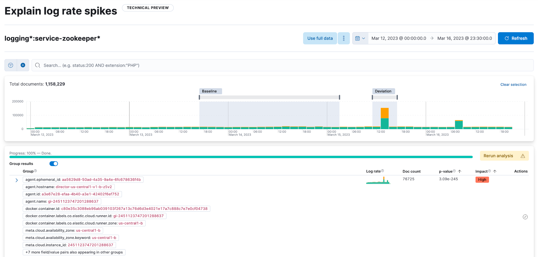
The use cases of frequent items are manifold. Yet the aggregation was not implemented for the analysis of shopping carts. As part of AIOps Labs, Explain Log Rate Spikes identifies reasons for increases in log rates. Frequent_item_sets is part of it. The decision to implement it as an aggregation makes other uses possible.
Choosing the base algorithm
Most famous and best known is the Apriori algorithm. Apriori builds candidate item sets breath first. It starts with building sets containing only one item and then expanding those sets in every iteration by one more item. After sets have been generated, they are tested against the data. Infrequent sets — those that do not reach a certain support, defined upfront — are pruned before the next iteration. Pruning might remove a lot of candidates, but the biggest weakness of this approach remains the requirement to keep a lot of item set candidates in memory.
Although the first prototypes of the aggregation used Apriori, it was clear from the beginning that we wanted to switch the algorithm later. We looked for one that better scales in runtime and memory. We decided on Eclat, other alternatives are FP-Growth and LCM. All three use a depth-first approach, which fits our resource model much better. Christian Borgelt’s overview paper has details about the various approaches and differences.
Fields and values
An Elasticsearch index consists of documents with fields and values. Values have different types, and each field can be an array of values. Translated to frequent item sets, a single item consists of exactly one field and one value. If a field stores an array of values, frequent_item_sets treats every value in the array as a single item. In other words, a document is a set of items. Yet not all fields are of interest; only the subset of fields used for frequent_item_sets is a transaction.
Dealing with distributed storage
Beyond choosing the main algorithm, other details required attention. The input data for an aggregation can be in one or many indices further separated in shards. In other words, data isn’t stored in one central place. This sounds like a weakness at first, but it has an advantage. At the shard level execution happens in parallel, so it makes sense to put as much as possible into the mapping phase.
Data preparation and mining basics
During mapping, items and transactions get de-duplicated. To reduce size, we encode items and transactions in big tables together with a counter. That counter later helps us to reduce runtime.
Once all shards have sent data to the coordinating node, the reduce phase starts with merging all shard results. In contrast to other aggregations, the main task of frequent_item_sets starts. Most of the runtime gets spent on generating and testing sets.
After the results are merged, we have a global view and can prune items. An item with a lower count than a minimum count gets dropped. Transactions might collapse as a result of item pruning. We calculate the minimum count using the minimum support parameter and the total document count:

Finding the top-N most frequent closed item sets
The minimum count has another use at runtime. Usually, it is not necessary to calculate all frequent item sets, but only a top-N, while N is given by the size parameter. Once the algorithm has found N frequent item sets, it raises the minimum count to the count of the weakest set. That way the bar raises and further mining can be skipped if the count of the candidate set gets below the bar.
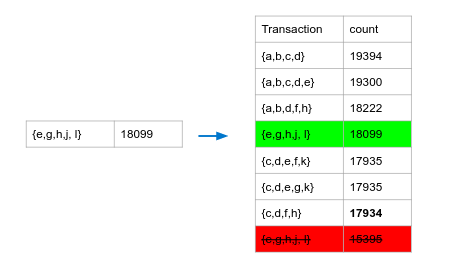
After pushing {e, g, h, j, l} into the fixed size queue, the minimum count is raised from 15395 to 17934.
Search order
Reducing the search space is key to reducing runtime. Simply generating every candidate set and testing it would be computationally heavy. To prune early, item sets are generated by taking single items with high counts first, in the hope of finding high count frequent sets earlier and hence increasing the adaptive minimum count. In Eclat, search is implemented as tree traversal over a prefix tree. This tree also ensures that candidate sets are visited exactly once.
Due to ordering the items by count, every additional item has a lower count than the previous one. This way the algorithm always knows whether a minimum count can be reached or not. In a similar fashion transaction counts are used, every transaction that does not match a candidate set reduces the reachable count.
Creating the candidate sets and testing them against transactions is the main driver of runtime. By using the techniques above, the implementation cuts the search space whenever possible. The original Apriori algorithm, in contrast, does not allow those short cuts.
Lookup tables and other tricks
Besides traversal order and early pruning, the implementation of frequent_item_sets uses a lot of low-level techniques to speed up mining. The deterministic order of items and transactions makes it possible to use bit vectors. One set bit represents the position of an item in the ordered list. The core of frequent_item_sets mainly uses those vectors and resolves results only at the very end. Similar bit vectors are used in other places to check for supersets. When scoring a candidate set, bit vectors are used to skip over transactions that have been ruled out earlier.
Lookup tables play a big role in successors of Apriori. Eclat uses them, and FP-Growth makes even more use of it for the price of higher memory requirements. In a nutshell, they do the usual search engine tradeoff between size and runtime. However, note that lookup tables can get large and must be carefully applied. In contrast to the versions found in academic papers, frequent_item_sets uses tables only for the top N items and up to a certain set size.
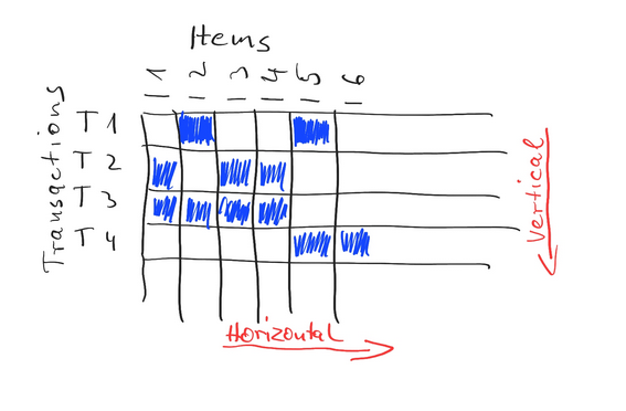
Lookup tables are bit matrices that can be organized vertically or horizontally. Vertically means storing for each item the transactions containing it. Horizontally organized bit vectors store for each transaction the items contained.
Circuit breaking and resource monitoring
Taking an academic paper and implementing it in production is interesting. Besides the problems mentioned above, a lot of other problems needed to be solved. Frequent_item_sets has to work for different kinds of data in different sizes. It is important that this aggregation does not impact other running tasks. All data structures support circuit breakers, ensuring that a request is stopped if it breaches a resource budget.
Using frequent items at scale
Despite all the optimizations mentioned, mining frequent item sets remains an expensive task. We recommend using async search. With async search, you can run the aggregation in the background and cancel it any time. Running frequent_item_sets as sub-aggregation next to random sampler reduces runtime. Some loss in precision doesn't matter at scale.
Another high impact on runtime performance are parameters. Results are not simply cut off using size. But size limits the search space and hence impacts runtime. Filters limit search space as well. The aggregation supports filtering documents and filtering of items via includes and excludes.
Progress, simple, perfection
Since frequent_item_sets shipped with 8.4, several enhancements have been implemented. Recently we discovered that especially machine generated data sometimes caused long run times. By implementing perfect extension pruning, we were able to improve runtime for some data sets. Perfect extensions are items that always co-occur. In future releases, we plan further improvements — a nightly benchmark monitors performance.
Conclusion
With frequent_item_sets, we implemented an advanced data mining algorithm as aggregation. It can find regularities in data. In the stack Explain Log Rate Spikes makes use of it. As aggregation, you can combine it with other parts of search and power your use cases. Try it out — Elastic Cloud is just a few clicks away.
Share
- Share on Twitter
Share on Twitter
- Share on LinkedIn
Share on LinkedIn
- Share on Facebook
Share on Facebook
- Share by Email
Share by Email
- Print this page
Print