Catching malware with Elastic outlier detection
The end of traditional anti-virus techniques
In the early days of detecting malicious software, it was possible for analysts to examine samples and uncover specific filenames, byte sequences, or strings that were characteristic of a particular malware and use that as a signature to detect subsequent infection. In recent years, the advent of open source malware (such as the infamous IoT botnet generator, Mirai) and automated exploit kits have caused an explosion in the number of malware variants. The AV Institute, an independent information security research organization in Germany, registers 350,000 new malware samples every day! In addition to an explosion of variants, malware authors are increasingly using obfuscation to bypass traditional anti-virus engine detection signatures.
Machine learning to the rescue?
As a result, it has become nearly impossible for anti-malware detection systems to keep up with the expanding number of new variants and obfuscation techniques by using only traditional methods. A number of research groups have proposed applying machine learning techniques to cope with the influx of new malicious programs.
The idea of applying machine learning to detect malware is by no means new. Some of the earliest attempts to use machine learning techniques to detect the presence of malicious programs date to the 1990s, when a group of researchers at IBM used artificial neural networks to detect boot sector viruses. This technology was later incorporated into the IBM anti-virus engine.
Another way to approach a malware detection problem is to reframe it as an outlier detection problem. We assume that most of the binaries running on a given machine are benign and want to detect binaries that are outlying, since these could potentially be malicious. To perform outlier detection effectively, we have to analyze each binary to extract suitable features. Previous work in this area has used string counts, byte n-grams, and function call sequences as distinguishing features with some promising results.
Although results have been positive, the pace of research in this field is hampered by the lack of publicly available benchmark datasets. Security concerns related to the distribution of a large number of bundled malware and copyright issues have been the main blocker in making research datasets widely available.
The EMBER dataset
To help other research groups study the potential of machine learning algorithms in malware detection, Endgame Inc. released a publicly available dataset of features calculated from 1.1 million Portable Executable files (the format Windows operating systems use to execute binaries). Dubbed EMBER (Endgame Malware BEnchmark for Research), the open source classifier and dataset contains a mixture of known malicious, benign, and unlabeled files, which makes it ideal for use in classification and outlier detection experiments. Moreover, the dataset is labeled and thus perfect for evaluating the performance of an outlier detection algorithm. The labels have been generated by analyzing the file in VirusTotal — an online sandbox service that analyzes a file sample using a number of commercially available anti-virus engines.
As mentioned before, in order to perform outlier detection on binaries, we must first extract some features. The features in the EMBER dataset include string counts, average string lengths, the presence or absence of debug symbols, as well as byte count histograms. In a departure from previous work in this area, we decided to experiment with using byte histograms for outlier detection.
What are byte histograms? Each binary file can be represented as a sequence of bytes, which in decimal notation represent the values ranging from 0 to 255. A byte histogram is simply an array of values that describes the number of times each byte from 0 to 255 appears in the binary file. These counts are usually normalized to avoid any skews from overly large or small files.
Byte histogram fingerprints
Although to our knowledge, byte histograms have not been previously used in an outlier detection setting to detect malware, these are previous studies that indicate their utility in, for example, detecting whether or not a given malware binary has been obfuscated with a packer. Non-obfuscated binaries have uneven distributions of bytes while obfuscated binaries appear uniform. Given this interesting trait, we decided to investigate whether byte histograms could be used to distinguish between malicious and non-malicious binaries. A useful technique for quickly seeing whether a feature is useful for distinguishing between malicious and benign binaries is visualization.
To simultaneously visualize the byte histograms of the 300,000 malicious and 300,000 benign binaries, we plot the byte histograms as a grayscale image where the lighter the color of the pixel, the more of a given byte is present in the binary (see Figure 1).
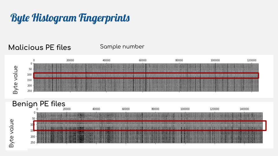
Comparing these two byte histogram fingerprints side by side, a few distinguishing features become obvious. The malicious binaries contain a higher proportion of byte histograms with severe irregularities, which appear as black lines in Figure 1. These samples have highly skewed proportions of bytes and are most likely encrypted or packed. Another distinguishing feature is the lightly shaded band that appears in the byte histogram fingerprint for benign binaries. It indicates that as a whole the benign binaries appear to have a higher concentration of bytes in the region 100-200 (see horizontal red band in Figure 1). This region is notably absent in the byte histogram fingerprint for the malicious binaries.
What could be the reason for this difference? The byte range 97-122 corresponds to the lowercase printable ASCII characters; in online discussions members of the security community suggested that the reason for the absence of this band in the malicious binaries is the heavy use of obfuscation, which tends to strip out printables to avoid detection. No such obfuscation is usually applied to benign binaries, hence the increased presence of printable ASCII characters.
Our visual inspection of the byte histogram fingerprints indicates differences in the byte compositions of malicious and benign files and suggests that byte histograms could potentially be used to detect a malicious file in a group of benign files.
Outlier detection algorithms
Given the promising results from our exploratory data analysis with byte histograms, we decided to see if our outlier detection algorithm (released as an experimental feature in 7.3) would be able to pick out malicious binaries from a mixed sample.
For our outlier detection technology, we use an ensemble of four well-established outlier detection techniques:
- Distance to kth nearest neighbor
- Average distance to k-nearest neighbors
- Local outlier factor
- Local density-based outlier factor
These first two algorithms give us global measures of how outlying a given point is, while the latter two measure how outlying a given point is with respect to the density of its neighbors. The full ensemble provides analysis of a given datapoint and outputs a final outlier score somewhere between 0 and 1. The closer a given datapoint scores to 1, the more outlying it is in a dataset.
In addition to an outlier score, we also compute a feature influence score. This is a numeric value that describes the contribution of each feature of a datapoint to the final outlier score and helps to interpret the results of the algorithm.
In the following sections, we will provide a practical walkthrough of our analysis of the EMBER dataset using Elastic outlier detection functionality.
A practical walkthrough of outlier detection
For the purposes of this demo, we will be using the Python library requests to interact with the Elasticsearch REST API and the elasticsearch-py library to extract the results of our analysis. All code examples will use Python 3.
First, we have to create an analytics job. We have ingested the documents that make up the dataset into a separate index called ember-malware and will use this as the source index to start our outlier detection analytics jobs. One good thing to keep in mind about outlier detection is that the algorithm operates on the assumption that the outliers, in our case the malicious binaries, make up a small proportion of the overall data population. Because the original dataset contains an equal proportion of malicious and benign samples, we downsample the malicious examples in the dataset so that the final dataset contains 300,000 benign samples and 3,000 malicious sample.
In addition to the source index, we will also need to supply a name for the destination index — this will be the index that will contain our original data and the results from the outlier detection analysis.
In the analysis block of the configuration, we can tweak the settings of the detector. By default, we will only write out feature influence scores for datapoints that have an outlier score of higher than 0.1. In this case, however, we want to examine the feature influence scores of all of our data points, so we will have to adjust feature_influence_threshold setting accordingly.
Finally, we want to adjust which fields of each datapoint are included in the analysis. By default, the outlier detection algorithm will analyze all numeric fields present in a given document in the source index. Since our dataset also includes a numeric label, which denotes whether a given datapoint is malicious or benign, we will need to exclude them from the analysis using the excludes array in the configuration. For a full explanation of all of the configuration options available, take a look at the documentation.
def create_outlier_detection(job_id, source_index, dest_index, host='http://localhost', port='9200'):
    host_config = f'{host}:{port}'
    url = f'/_ml/data_frame/analytics/{job_id}'
    config = {
        "source": {
            "index": f'{source_index}',
        },
        "dest": {
            "index": f'{dest_index}'
        },
        "model_memory_limit" : "3gb",
        "analysis": {
            "outlier_detection": {
      "feature_influence_threshold" : 0.0
    }
        },
        "analyzed_fields": {
            "excludes" : ["label"]
        }
    }
    print(requests.put(host_config+url, json=config).json())
After the job has been created, we can start it by posting a request to the start API endpoint.
def run_outlier_detection(job_id, host='http://localhost', port='9200'):
    host_config = f'{host}:{port}'
    url = f'/_ml/data_frame/analytics/{job_id}/_start'
    print(requests.post(host_config+url).json())
The runtime of the outlier detection analytics job will depend on the properties of the hardware your Elasticsearch cluster is running, on the number of documents in your source index, and on the number of fields each document has. It is possible to query the status of the outlier detection job by sending a request to the stats API endpoint.
def stats_outlier_detection(job_id, host='http://localhost', port='9200'):
    host_config = f'{host}:{port}'
    url = f'/_ml/data_frame/analytics/{job_id}/_stats'
    results = requests.get(host_config+url)
    return results.json()
Once the outlier detection analysis job has been completed, its status will be set to stopped and we can start exploring the results.
Exploring outlier detection results
After the outlier detection analysis has been completed, we can query the destination index for the results of the analysis. As mentioned before, the destination index will contain the original data, the outlier scores for each document and the feature influence values for each field in a document. We can export these results for further analysis into a Pandas dataframe using the helper functions in elasticsearch-py.
sha256_sums = []
outlier_scores = []
es_client = Elasticsearch()
for r in helpers.scan(es_client, index='dest_index'):
    sha256_sums.append((r['_source']['sha256'])
    outlier_scores.append(r['_source']['ml']['outlier_score'])
df_outlier_results = pd.DataFrame.from_dict({'sha256': sha256_sums, 'outlier_score': outlier_scores})
As a first exploratory step we want to sort our results in order of descending outlier score to see which binaries have scored the highest and to check if these high-scoring outliers are actually malicious.
Table 1: Top five most outlying binaries
SHA 256 checksum | Outlier score | VirusTotal status |
60314195b451333bd8de0818368611c5b0ab011ef0b169499198d036f0feb9cf | 0.871 | |
1c4df47a1d210a0c0356303b9cf5c9b2c8459474d46e05e6fad1eb74f89248ab | 0.863 | |
774dfa148dbc2a6f38484040c99f57c7aee5e921e696f6ae6d71fd7310df5479 | 0.844 | |
90ff7bb166c7e94b1fe72fa1bcbcf753946d67f98aaedf194579653ee84abc6e | 0.838 | |
186fcaff37451ab3b3da44f946222592153a1169e1357b07f28e2cd3010ae4e1 | 0.836 |
As we can see from Table 1, four out of the five most outlying binaries identified by the outlier detection process are malicious Windows Trojans.
To get a more comprehensive view of how the byte histogram fingerprint profiles correlate with the outlier score, we can sort all of our binaries in order of increasing outlier score and plot out another byte histogram fingerprint (see Figure 2) for the dataset. The vertical axis denotes the byte, while the horizontal one tracks the number of the binary sample. The shading indicates the frequency of the byte present in a sample. Lighter shades correspond to a higher frequency. The samples are ordered by ascending outlier score. Those on the left are the most normal, while those on the very right, the most outlying. Examining the figure, we notice that the individual byte histograms tend to become more and more irregular as we move in the direction of increasing outlier score.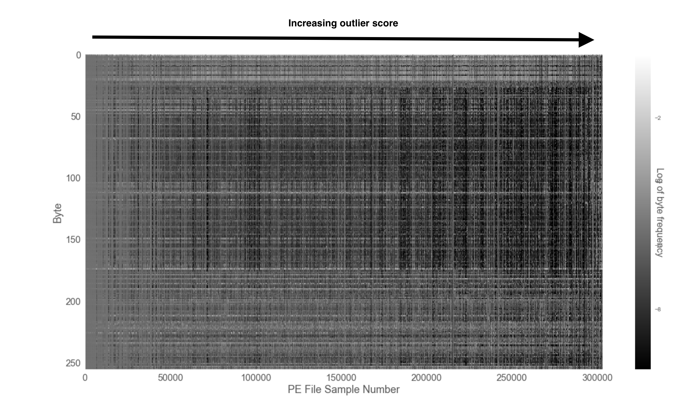
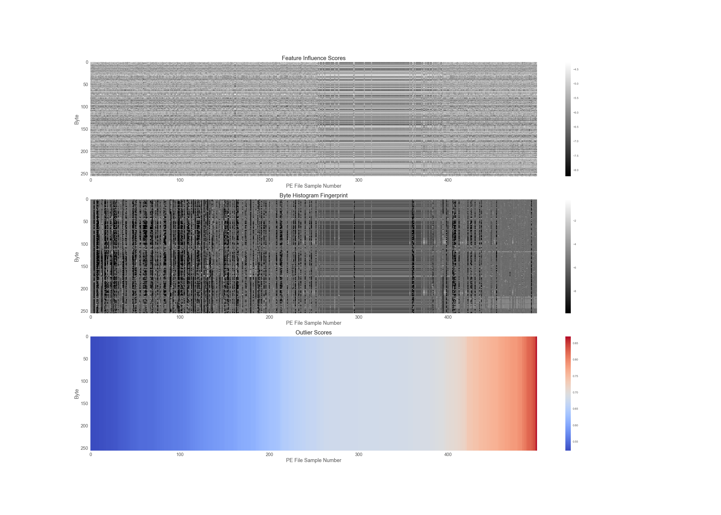
In addition, to outlier scores, we can also examine the feature influence values of each byte frequency in a sample to see which bytes are the most important in deciding whether a binary is an outlier or inlier. In Figure 3, we have plotted the feature influence scores, the byte histogram frequencies and the outlier scores of the 500 most outlying binaries in our dataset.
Using the Evaluate API to evaluate outlier detection
In addition to analytics functions, we also provide an Evaluate API that can compute standard industry metrics such as confusion matrices, precision, recall, and the receiver-operating characteristics curve to evaluate outlier detection results. These metrics tell users how well our outlier detection algorithm performs against a dataset, which is marked up with the true outliers. In the case of EMBER, we know which samples correspond to malware and which to benign binaries and thus we can compare the labels in the dataset to the results from the outlier detection analysis.
Let’s see how to use the Evaluate API to evaluate the results of the outlier detection analysis on the EMBER dataset.
First, we must make sure that the index that contains our classification results also contains a field with the ground truth label. In our case, this field is simply called label and we supply it in the configuration’s actual_field block (see example in code sample below). In addition to the ground truth label, we need to supply a field that contains the results of our algorithm’s predictions. In the case of outlier detection, these predictions are the outlier scores and are stored in the ml.outlier_score field.
def evaluate_outlier_detection(dest_index, host='http://localhost', port='9200', label_field='label'):
    host_config = f'{host}:{port}'
    url = f'/_ml/data_frame/_evaluate'
    config = {
      "index": f'{dest_index}',
      "evaluation": {
        "binary_soft_classification": {
          "actual_field": f'{label_field}',
          "predicted_probability_field": "ml.outlier_score",
          "metrics": {
        "auc_roc": {
          "include_curve": True
        },
        "precision": { "at": [0.25, 0.50, 0.75] },
        "recall": { "at": [ 0.25, 0.50, 0.75 ] },
        "confusion_matrix": { "at": [ 0.25, 0.50, 0.75 ] }
        }
      }
    }
    }
    result_dict = requests.post(host_config+url, json=config).json()
    return result_dict
Last, but not least, we need to supply thresholds in our evaluation configuration. Because the outlier detection algorithm outputs a continuous numerical score instead of a binary classification label, we have to select a threshold to binarize these results. For example, we could say that all datapoints that have an outlier score of greater than or equal to 0.75 are considered outliers and all points that score below are inliers. The choice of this threshold is slightly arbitrary, so we can supply a range of values to see how the classification results change as we manipulate the threshold.
The Evaluate API will return our requested evaluation metrics in the response.
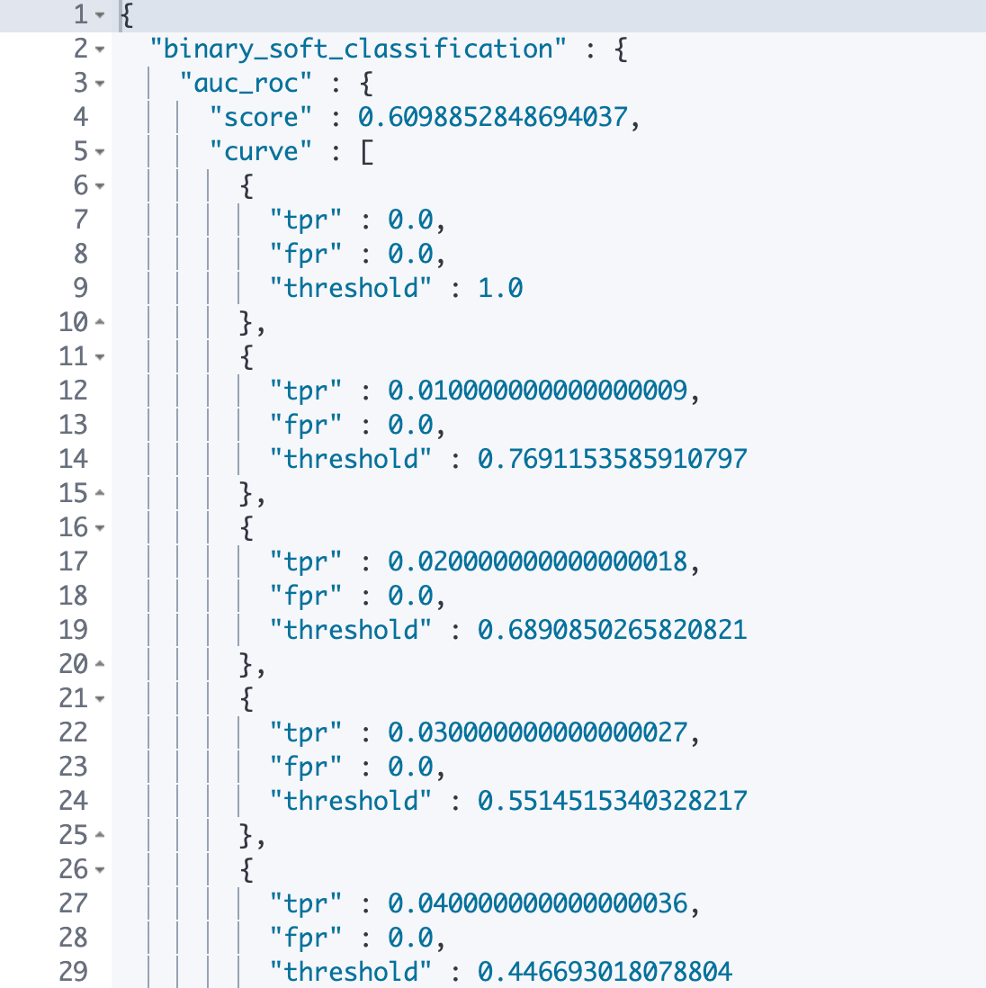
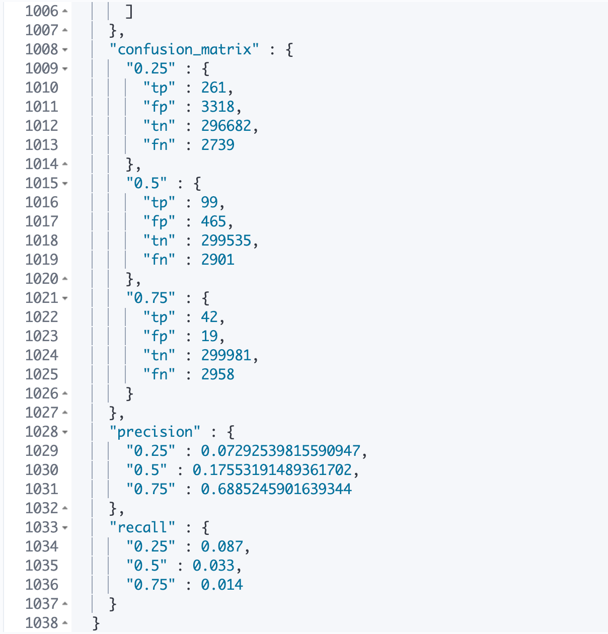
As we can see from Figure 4, the Evaluate API has computed performance metrics such as precision and recall for our outlier detection algorithm at each of the thresholds we supplied. We have also received back the entire receiver operating characteristics curve and the area under the curve. The area gives us a single summarized measure of how well outlier detection performs across a range of thresholds. The closer this value is to 1, the better the performance of the algorithm is overall.
For our malware detection analysis, the area is 0.61, which suggests some further room for improvement in the way we downsample our dataset or in the features we choose for outlier detection. Perhaps we could use some additional features from binary files such as string counts to improve our outlier detection results.
Choosing a suitable decision threshold
While in our evaluation step, we are interested in getting an aggregate view of outlier detection performance at various thresholds, for practical purposes we might often want to choose a single decision threshold to determine which samples are outliers and which are inliers. How does one, then, choose a suitable threshold for outlier detection?
The answer depends on the false positive tolerance of your outlier detection usecase. What do we mean by that? Let’s think back to our problem of catching malware using outlier detection. If we set the threshold very low, let’s say at 0.2, we would end up classifying many of the binaries we examine as “outliers”. We would end up catching lots of malware, but also more benign programs would be mistakenly classified as outlying.
Alternatively, we could raise the threshold and consider only those binaries that score above 0.75 to be outlying. We would reduce the number of benign programs mistakenly classified as outlying, but there is now a higher chance we would let through a program that is truly malicious. Therefore, in this case, the choice of decision threshold depends on how risky it would be to mistakenly label a malicious program as normal versus how much trouble it would cause to mistakenly label a benign program as outlying. Perhaps, if we are running this analysis on a critical system, we might accept that some of our benign programs will be accidentally mislabeled as a suitable cost for making sure that no malicious program makes it through our detector and set the threshold low.
Conclusion
In today's world, traditional anti-virus signature techniques are struggling to keep up with the daily influx of new malware variants. Machine learning techniques have been suggested as a suitable aid in detecting and classifying these new malware variants and academic studies as well as industry labs have shown the promise of these techniques in practical applications.
In this analysis, we have used the new Elastic outlier detection functionality to see if we can use byte histogram profiles extracted from binaries to detect malware. Although by no means a panacea for malware detection, our results are promising and suggest that in the future machine learning techniques can be of significant use to malware analysts.