User annotations for Elastic machine learning
Editor's Note: With the release of Elastic Stack 7.11, the new alerting framework is now generally available. In addition to existing connectors to 3rd party platforms like Slack PagerDuty, and Servicenow, 7.11 adds Microsoft Teams to the list of built-in alerting integrations. Read more about this update in our alerting release blog.
User annotations are a new machine learning feature in Elasticsearch available from 6.6 onwards. They provide a way to augment your machine learning jobs with descriptive domain knowledge. When you run a machine learning job, its algorithm is trying to find anomalies — but it doesn’t know what the data itself is about. The job wouldn't know, for example, whether it was dealing with CPU usage or network throughput. User annotations offer a way to augment the results with the knowledge you as a user have about the data.
In this blog post, we’ll show you how user annotations work and how to apply them to different use cases. We’ll be analysing data from Hydro Online — an open data portal run by Austria’s Tyrolean local government. Hydro Online offers an interface to investigate weather sensor data such as rainfall accumulation, river height, or snowpack totals. As described in one of our previous blog posts, the File Data Visualizer offers a robust way to ingest data from CSV data, as is found in this case.
Usage
Let’s start with a single metric job that analyses river height measurements of the River Grossache going through the village of Kössen. Once the job is created, the Single Metric Viewer can be used to add annotations to the results of the analysis. Simply drag over a time range in the chart to create an annotation. A flyout element will pop up to the right, which allows you to add a custom description. In the example below, we annotate an anomalous river height (a major flooding occurred on that date). By creating the annotation, you can make that knowledge available to other users.
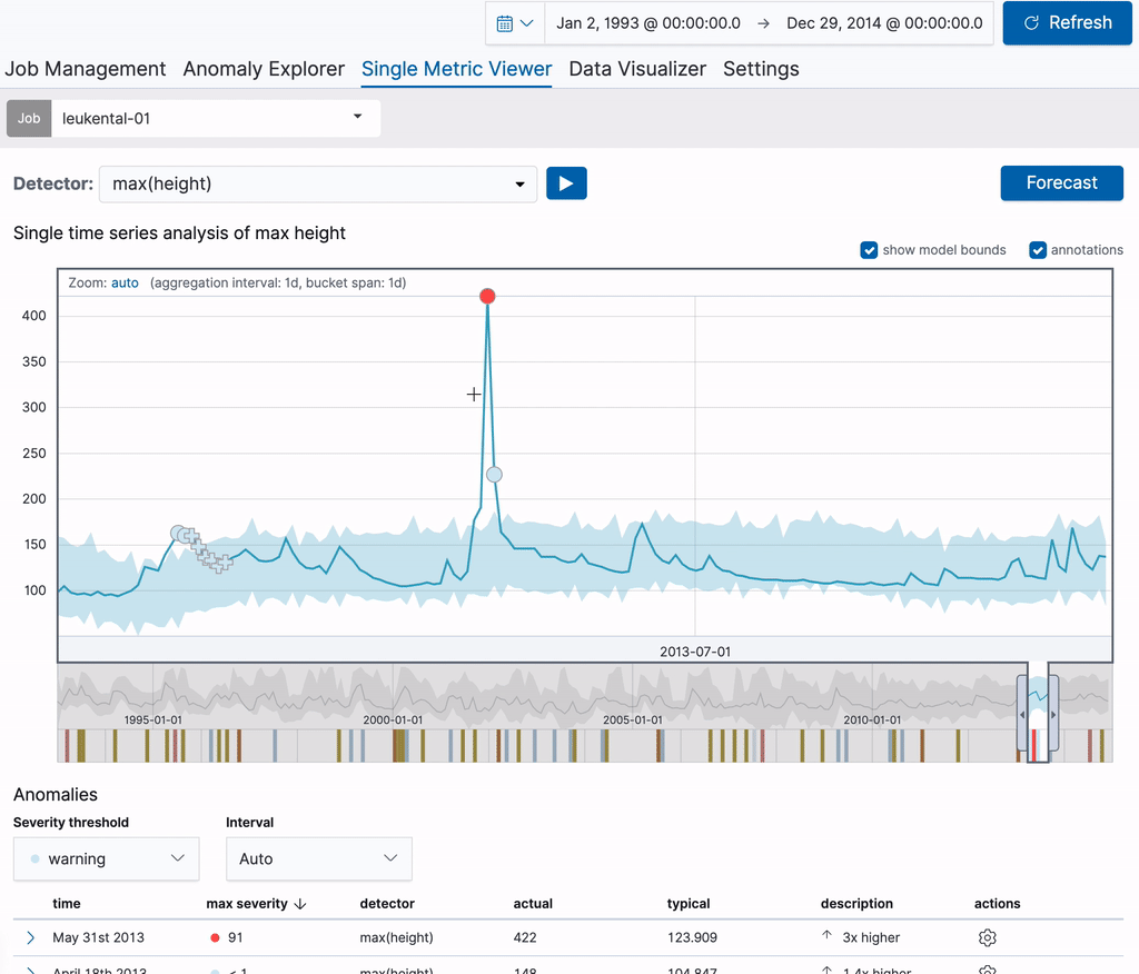
The annotation is visible in both the chart itself as well as in the Annotations table below it. The label visible in the first column of the table can be used to identify the annotation in the chart. These labels are dynamically created for the annotations on display. When hovering over a row in the Annotations table, the corresponding annotation will also be highlighted in the chart above it.
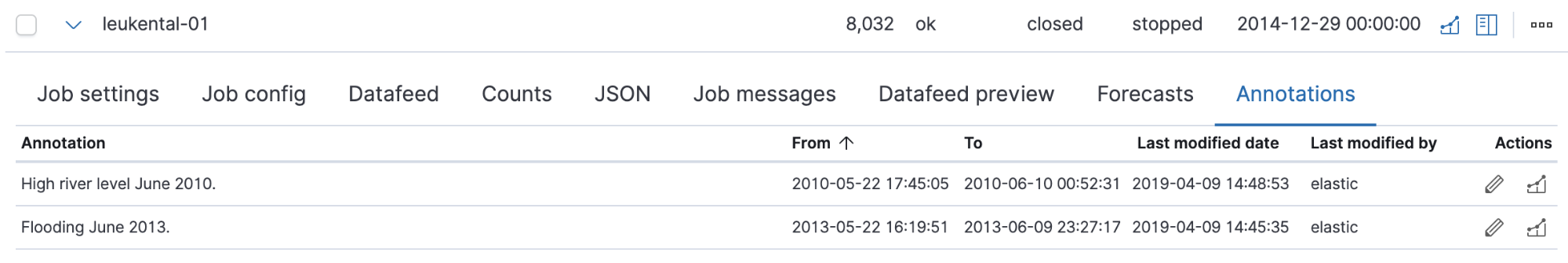
The annotations created for each job can also be accessed from the Job Management page, where they are displayed in their own tab by expanding a row in the list of jobs. Each annotation in the table includes a link in the right hand column, which takes you back to the Single Metric Viewer with a focus on the time range covered by the annotation. These permalinks can also be shared with others. This means you can use annotations to create bookmarks on particular anomalies to revisit them later on.
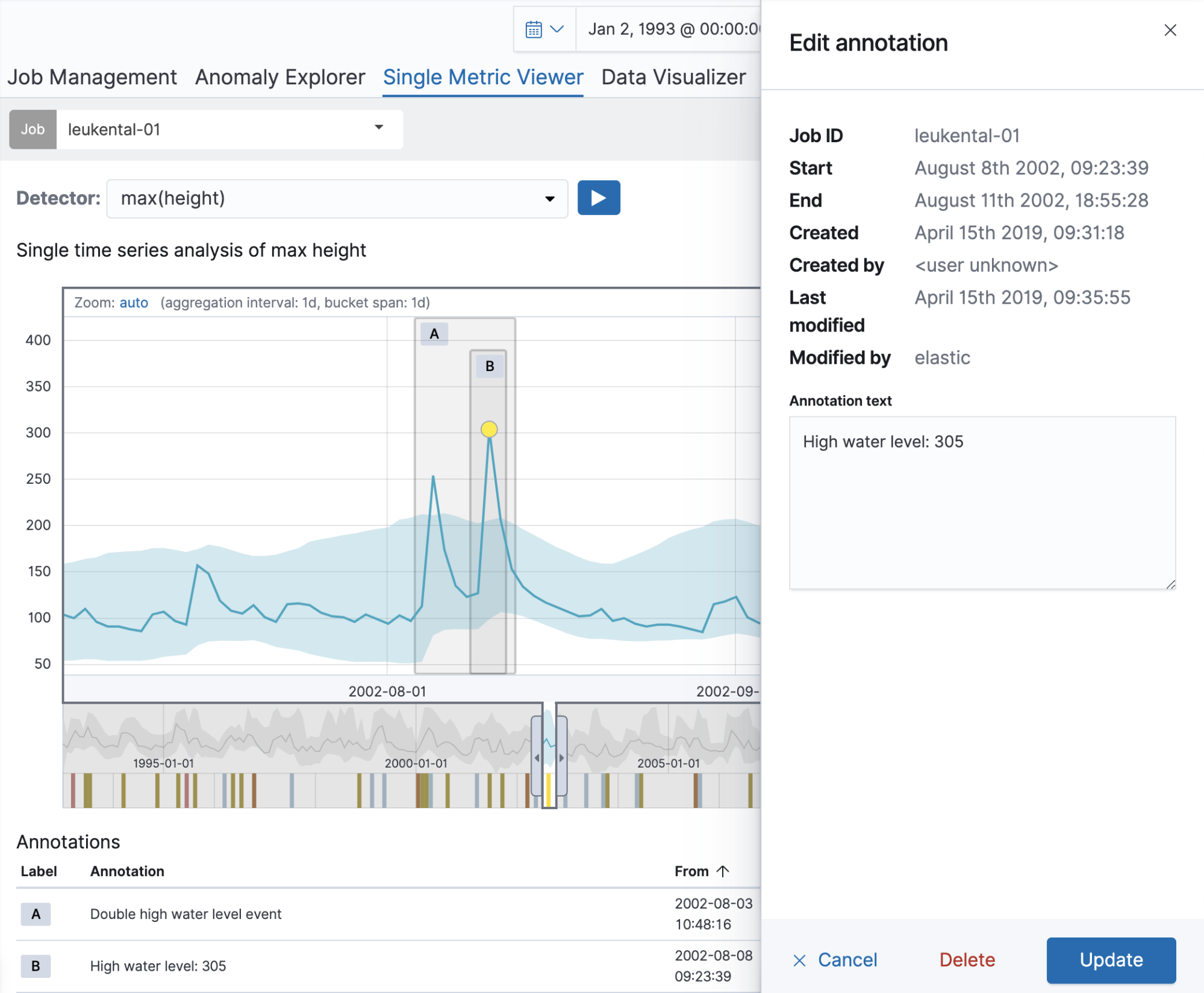
If there are multiple annotations covering the same time range, annotations will be vertically distributed in the chart to avoid overlap. To edit or delete an annotation, simply click on it in the chart. The flyout element will open again to the right where you’ll be able to edit the text or delete the annotation. From 6.7 onwards, this can also be done by using the edit button in the Annotations table, making this functionality available from the Job Management page too.
Now that we've covered the basic functionality of how to create and work with user annotations, let's move on to some more use cases.
Using annotations to verify expected anomalies
Annotations can be used to supply a ground truth to verify if a machine learning job comes up with expected results. In the following example, we are again looking at the river level data from Hydro Online and are now aiming to automatically overlay historic events as annotations on the anomaly results. As a data scientist, for example, your work might include obtaining and preparing both the source data you want to analyse as well as the data set to verify the results.
For our own analysis, we need the raw dataset.
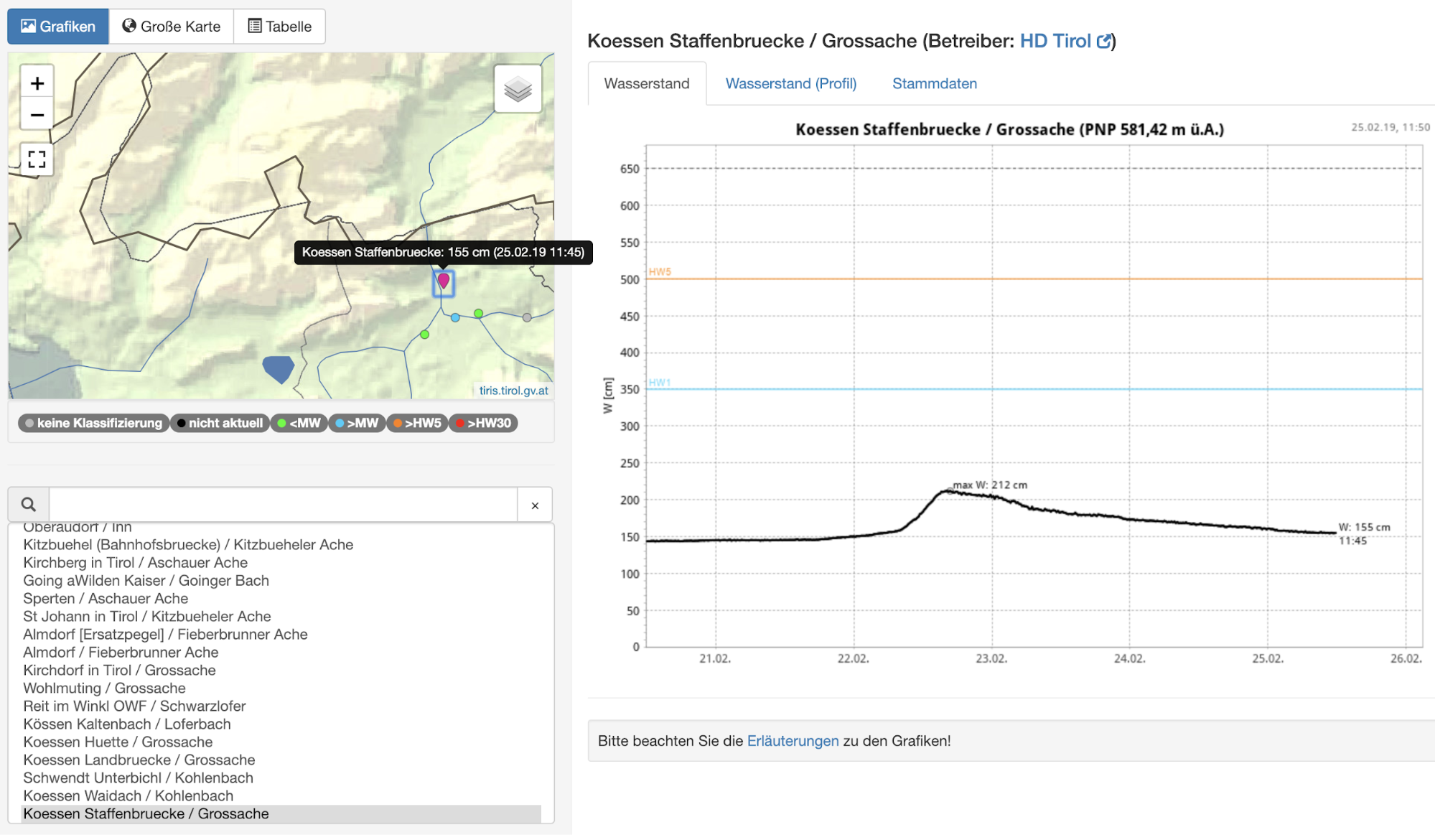
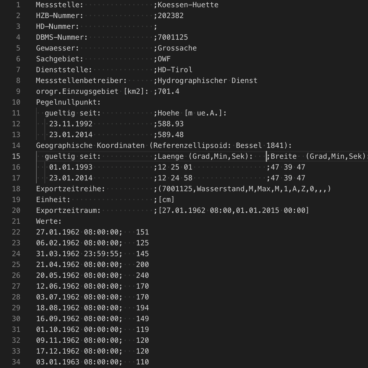
Luckily, in this case, in addition to investigating data via the web interface, we can also download historic data for further analysis. For this example we’ll use the river height data of the River Grossache measured at the “Huette” measurement point. The annotations covering the desired ground truth will be created from a document describing severe river heights and floods.
|

|
In addition to using the UI previously described, machine learning annotations are stored as documents in a separate standard Elasticsearch index. Annotations can also be created programmatically or manually using standard Elasticsearch APIs. Annotations are stored in a version-specific index, and should be accessed via the aliases .ml-annotations-read and .ml-annotations-write. For this example, we'll add annotations to reflect the historic river events before creating our machine learning job.
{
   "_index":".ml-annotations-6",
   "_type":"_doc",
   "_id":"DGNcAmoBqX9tiPPqzJAQ",
   "_score":1.0,
   "_source":{
      "timestamp":1368870463669,
      "end_timestamp":1371015709121,
      "annotation":"2013 June; 770 m3/s; 500 houses flooded.",
      "job_id":"annotations-leukental-4d-1533",
      "type":"annotation",
      "create_time":1554817797135,
      "create_username":"elastic",
      "modified_time":1554817797135,
      "modified_username":"elastic"
   }
}
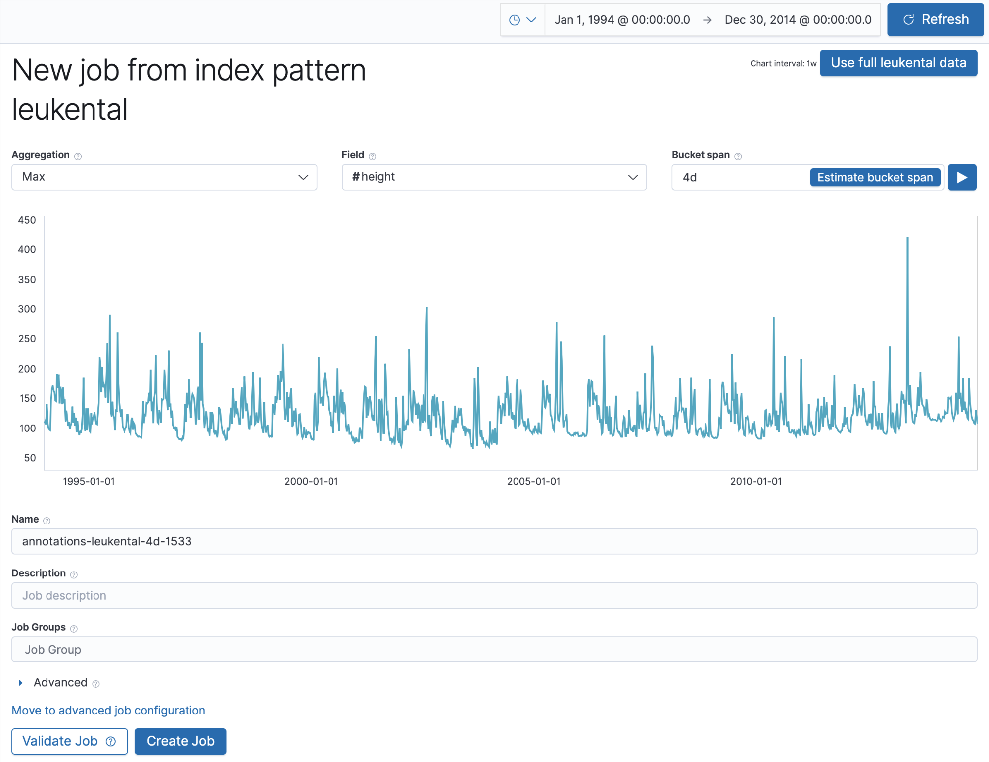
We’ll now create a machine learning job to find anomalies in maximum river height using a name that matches the job_id field from the annotation above so that it picks up the manually created annotations. This is how this job looks in the Single Metric wizard once we ingest the historic river data into an Elasticsearch index:
The important bit here is that the job name we chose matches the one used for the annotations. Once we run the job and move to the Single Metric Viewer, we should see annotations corresponding to the anomalies in river height that the machine learning job detected:
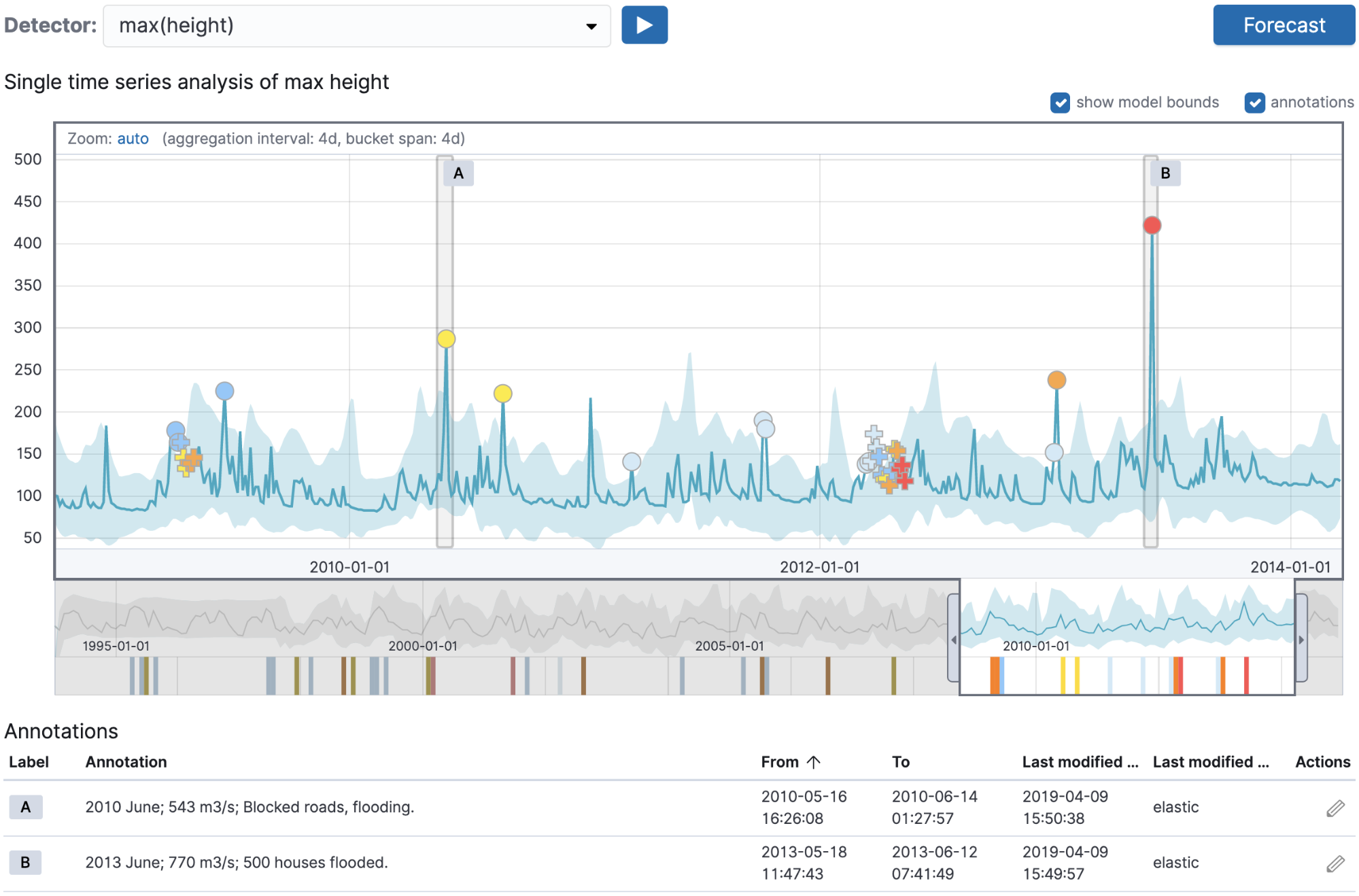
This technique offers a great way to verify if the analysis you’re running is valid when compared to pre-existing validation data stored as annotations.
Annotations for system events
In addition to the user-generated annotations above, the machine learning backend automatically creates annotations in some circumstances for system events.
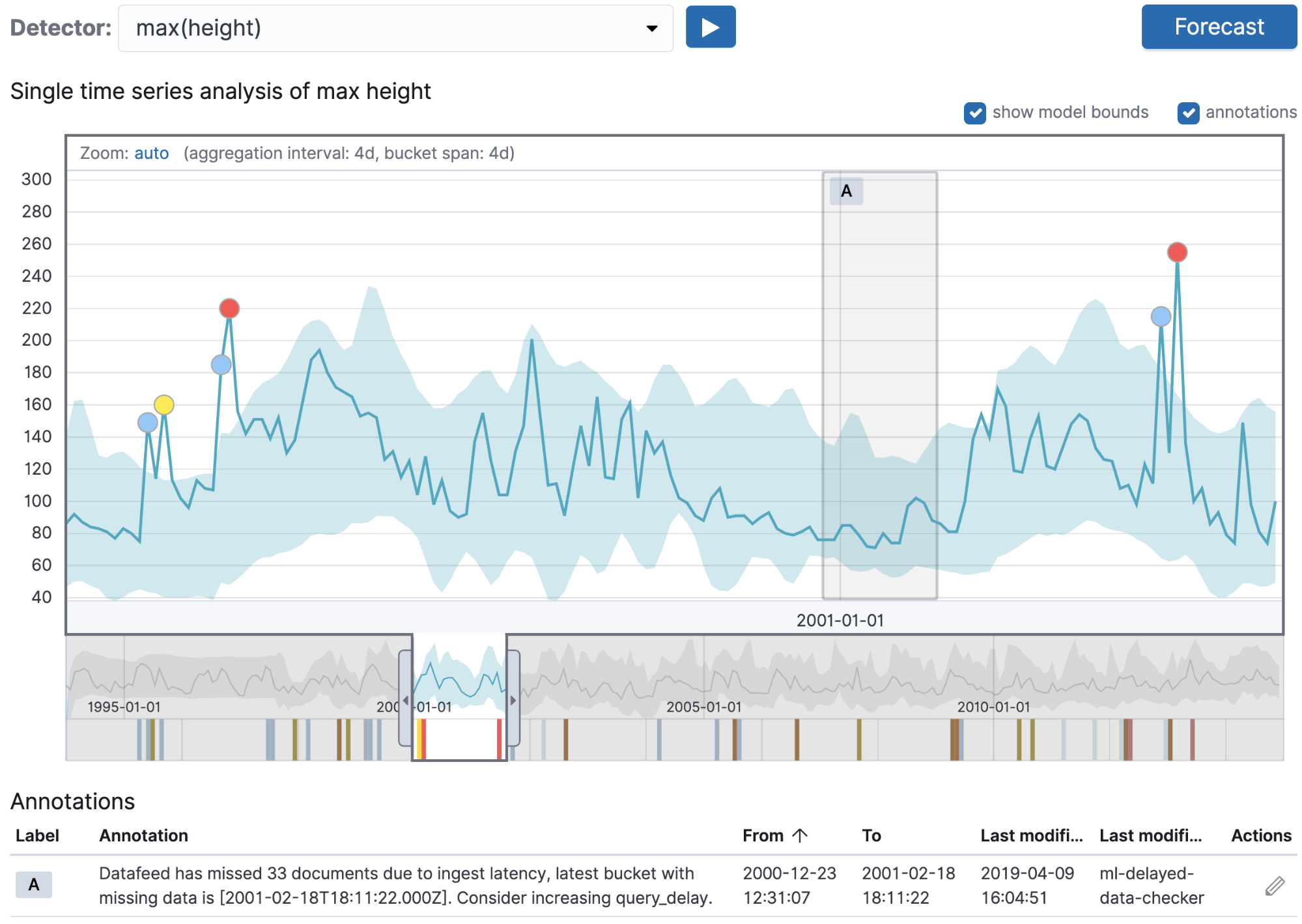
The screenshot above shows an example of an automatically created annotation. In this case, a real-time machine learning job was run, but data ingestion wasn’t able to keep up with the ingestion rate required for the job. This meant documents were added to the index after the job had run its analysis on the bucket. The automatically created annotation highlights this issue that was previously hard to spot and debug. The annotation text features detail the identified problem and provide a suggestion on how to solve it — in this case increasing the query_delay setting.
Alerting integration
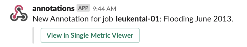
Even before the availability of user annotations for machine learning, you could use Watcher to create alerts based on anomalies identified by machine learning jobs. While that is a great improvement when compared to alerting on basic thresholds, the alerts may be too granular for the target group that receives the alerts. As a user of machine learning jobs, annotations can give you a way to curate what gets triggered as Watcher alerts and what gets passed on to other stakeholders. Since annotations are stored in their own Elasticsearch index, you can use Watcher to simply react to newly created documents in that index and trigger notifications. Watcher can also be configured to send alerts to a Slack channel. The following configuration gives you an example on how to create a watch to trigger Slack messages when a new annotation gets created:
{
 "trigger": {
   "schedule": {
     "interval": "5s"
   }
 },
 "input": {
   "search": {
     "request": {
       "search_type": "query_then_fetch",
       "indices": [
         ".ml-annotations-read"
       ],
       "rest_total_hits_as_int": true,
       "body": {
         "size": 1,
         "query": {
           "range": {
             "create_time": {
               "gte": "now-9s"
             }
           }
         },
         "sort": [
           {
             "create_time": {
               "order": "desc"
             }
           }
         ]
       }
     }
   }
 },
 "condition": {
   "compare": {
     "ctx.payload.hits.total": {
       "gte": 1
     }
   }
 },
 "actions": {
   "notify-slack": {
     "transform": {
       "script": {
         "source": "def payload = ctx.payload; DateFormat df = new SimpleDateFormat(\"yyyy-MM-dd'T'HH:mm:ss.SSS'Z'\"); payload.timestamp_formatted = df.format(Date.from(Instant.ofEpochMilli(payload.hits.hits.0._source.timestamp)));  payload.end_timestamp_formatted = df.format(Date.from(Instant.ofEpochMilli(payload.hits.hits.0._source.end_timestamp))); return payload",
         "lang": "painless"
       }
     },
     "throttle_period_in_millis": 10000,
     "slack": {
       "message": {
         "to": [
           "#<slack-channel>"
         ],
         "text": "New Annotation for job *{{ctx.payload.hits.hits.0._source.job_id}}*: {{ctx.payload.hits.hits.0._source.annotation}}",
         "attachments": [
           {
             "fallback": "View in Single Metric Viewer http://<kibana-host>:5601/app/ml#/timeseriesexplorer?_g=(ml:(jobIds:!({{ctx.payload.hits.hits.0._source.job_id}})),refreshInterval:(pause:!t,value:0),time:(from:'{{ctx.payload.timestamp_formatted}}',mode:absolute,to:'{{ctx.payload.end_timestamp_formatted}}'))&_a=(filters:!(),mlSelectInterval:(interval:(display:Auto,val:auto)),mlSelectSeverity:(threshold:(color:%23d2e9f7,display:warning,val:0)),mlTimeSeriesExplorer:(zoom:(from:'{{ctx.payload.timestamp_formatted}}',to:'{{ctx.payload.end_timestamp_formatted}}')),query:(query_string:(analyze_wildcard:!t,query:'*')))",
             "actions": [
               {
                 "name": "action_name",
                 "style": "primary",
                 "type": "button",
                 "text": "View in Single Metric Viewer",
                 "url": "http://<kibana-host>:5601/app/ml#/timeseriesexplorer?_g=(ml:(jobIds:!({{ctx.payload.hits.hits.0._source.job_id}})),refreshInterval:(pause:!t,value:0),time:(from:'{{ctx.payload.timestamp_formatted}}',mode:absolute,to:'{{ctx.payload.end_timestamp_formatted}}'))&_a=(filters:!(),mlSelectInterval:(interval:(display:Auto,val:auto)),mlSelectSeverity:(threshold:(color:%23d2e9f7,display:warning,val:0)),mlTimeSeriesExplorer:(zoom:(from:'{{ctx.payload.timestamp_formatted}}',to:'{{ctx.payload.end_timestamp_formatted}}')),query:(query_string:(analyze_wildcard:!t,query:'*')))"
               }
             ]
           }
         ]
       }
     }
   }
 }
}
In the configuration above, just replace <slack-channel> and <kibana-host> with your settings and use it to create an advanced watch. Once everything is set up, you should receive a Slack notification every time you create a new annotation — including the annotation text and a link back to Single Metric Viewer.
Summary
In this article we introduced the new annotations feature for Elasticsearch machine learning. It can be used for adding annotations via the UI and for system annotations triggered via backend tasks. These annotations are available as bookmarks via the Job Management page and are sharable as links with others. Annotations can be created programmatically from external data to be used as a ground truth overlay for detected anomalies. Finally, in combination with Watcher and the slack action in Elasticsearch, we’ve seen how annotations can be used for curated alerting. Have fun with annotations, and find us on the Discuss forums if you have any questions.