Predicting numerical values with regression
editPredicting numerical values with regression
editRegression analysis is a supervised machine learning process for estimating the relationships among different fields in your data, then making further predictions on numerical data based on these relationships. For example, you can predict the response time of a web request or the approximate amount of data that the server exchanges with a client based on historical data.
When you perform regression analysis, you must identify a subset of fields that you want to use to create a model for predicting other fields. Feature variables are the fields that are used to create the model. The dependent variable is the field you want to predict.
Regression algorithms
editRegression uses an ensemble learning technique called extreme gradient boost (XGboost) which combines decision trees with gradient boosting methodologies.
There are three types of feature variables that you can use with these algorithms: numerical, categorical, or Boolean. Arrays are not supported.
1. Define the problem
editRegression can be useful in cases where a continuous quantity needs to be predicted. The values that regression analysis can predict are numerical values. If your use case requires predicting continuous, numerical values, then regression might be the suitable choice for you.
2. Set up the environment
editBefore you can use the Elastic Stack machine learning features, there are some configuration requirements (such as security privileges) that must be addressed. Refer to Setup and security.
3. Prepare and transform data
editRegression is a supervised machine learning method, which means you need to supply a labeled training data set. This data set must have values for the feature variables and the dependent variable which are used to train the model. This information is used during training to identify relationships among the various characteristics of the data and the predicted value. This labeled data set also plays a critical role in model evaluation.
You might also need to transform your data to create a data frame which can be used as the source for regression.
To learn more about how to prepare your data, refer to the relevant section of the supervised learning overview.
4. Create a job
editData frame analytics jobs contain the configuration information and metadata necessary to perform an analytics task. You can create data frame analytics jobs via Kibana or using the create data frame analytics jobs API.
Select regression as the analytics type for the job, then select the field that you want to predict (the dependent variable). You can also include and exclude fields to/from the analysis.
5. Start the job
editYou can start the job via Kibana or using the start data frame analytics jobs API. A regression job has the following phases:
-
reindexing: Documents are copied from the source index to the destination index. -
loading_data: The job fetches the necessary data from the destination index. -
feature_selection: The process identifies the most relevant analyzed fields for predicting the dependent variable. -
coarse_parameter_search: The process identifies initial values for undefined hyperparameters. -
fine_tuning_parameters: The process identifies final values for undefined hyperparameters. Refer to hyperparameter optimization. -
final_training: The model training occurs. -
writing_results: The job matches the results with the data rows in the destination index, merges them, and indexes them back to the destination index. -
inference: The job validates the trained model against the test split of the data set.
After the last phase is finished, the job stops and the results are ready for evaluation.
When you create a data frame analytics job, the inference step of the process might fail if the model is too large to fit into JVM. For a workaround, refer to this GitHub issue.
6. Evaluate the result
editUsing the data frame analytics features to gain insights from a data set is an iterative process. After you defined the problem you want to solve, and chose the analytics type that can help you to do so, you need to produce a high-quality data set and create the appropriate data frame analytics job. You might need to experiment with different configurations, parameters, and ways to transform data before you arrive at a result that satisfies your use case. A valuable companion to this process is the evaluate data frame analytics API, which enables you to evaluate the data frame analytics performance. It helps you understand error distributions and identifies the points where the data frame analytics model performs well or less trustworthily.
To evaluate the analysis with this API, you need to annotate your index that contains the results of the analysis with a field that marks each document with the ground truth. The evaluate data frame analytics API evaluates the performance of the data frame analytics against this manually provided ground truth.
You can measure how well the model has performed on your training data by using
the regression evaluation type of the
evaluate data frame analytics API. The
mean squared error (MSE) value that the evaluation
provides you on the training data set is the training error. Training and
evaluating the model iteratively means finding the combination of model
parameters that produces the lowest possible training error.
Another crucial measurement is how well your model performs on unseen data. To assess how well the trained model will perform on data it has never seen before, you must set aside a proportion of the training set for testing (testing data). Once the model is trained, you can let it predict the value of the data points it has never seen before and compare the prediction to the actual value. This test provides an estimate of a quantity known as the model generalization error.
The regression evaluation type offers the following metrics to evaluate the model performance:
- Mean squared error (MSE)
- Mean squared logarithmic error (MSLE)
- Pseudo-Huber loss
- R-squared (R2)
Mean squared error
editMSE is the average squared sum of the difference between the true value and the predicted value. (Avg (predicted value-actual value)2).
Mean squared logarithmic error
editMSLE is a variation of mean squared error. It can be used for cases when the target values are positive and distributed with a long tail such as data on prices or population. Consult the Loss functions for regression analyses page to learn more about loss functions.
Pseudo-Huber loss
editPseudo-Huber loss metric
behaves as mean absolute error (MAE) for errors larger than a predefined value
(defaults to 1) and as mean squared error (MSE) for errors smaller than the
predefined value. This loss function uses the delta parameter to define the
transition point between MAE and MSE. Consult the
Loss functions for regression analyses page to learn more about loss functions.
R-squared
editR-squared (R2) represents the goodness of fit and measures how much of the variation in the data the predictions are able to explain. The value of R2 are less than or equal to 1, where 1 indicates that the predictions and true values are equal. A value of 0 is obtained when all the predictions are set to the mean of the true values. A value of 0.5 for R2 would indicate that the predictions are 1 - 0.5(1/2) (about 30%) closer to true values than their mean.
Feature importance
editFeature importance provides further information about the results of an analysis and helps to interpret the results in a more subtle way. If you want to learn more about feature importance, click here.
7. Deploy the model
editThe model that you created is stored as Elasticsearch documents in internal indices. In other words, the characteristics of your trained model are saved and ready to be deployed and used as functions. The inference feature enables you to use your model in a preprocessor of an ingest pipeline or in a pipeline aggregation of a search query to make predictions about your data.
Inference
editInference is a machine learning feature that enables you to use supervised machine learning processes – like regression or classification – not only as a batch analysis but in a continuous fashion. This means that inference makes it possible to use trained machine learning models against incoming data.
For instance, suppose you have an online service and you would like to predict whether a customer is likely to churn. You have an index with historical data – information on the customer behavior throughout the years in your business – and a classification model that is trained on this data. The new information comes into a destination index of a continuous transform. With inference, you can perform the classification analysis against the new data with the same input fields that you’ve trained the model on, and get a prediction.
Inference processor
editInference can be used as a processor specified in an ingest pipeline. It uses a trained model to infer against the data that is being ingested in the pipeline. The model is used on the ingest node. Inference pre-processes the data by using the model and provides a prediction. After the process, the pipeline continues executing (if there is any other processor in the pipeline), finally the new data together with the results are indexed into the destination index.
Check the inference processor and the machine learning data frame analytics API documentation to learn more about the feature.
Inference aggregation
editInference can also be used as a pipeline aggregation. You can reference a trained model in the aggregation to infer on the result field of the parent bucket aggregation. The inference aggregation uses the model on the results to provide a prediction. This aggregation enables you to run classification or regression analysis at search time. If you want to perform the analysis on a small set of data, this aggregation enables you to generate predictions without the need to set up a processor in the ingest pipeline.
Check the inference bucket aggregation and the machine learning data frame analytics API documentation to learn more about the feature.
If you use trained model aliases to reference your trained model in an inference processor or inference aggregation, you can replace your trained model with a new one without the need of updating the processor or the aggregation. Reassign the alias you used to a new trained model ID by using the Create or update trained model aliases API. The new trained model needs to use the same type of data frame analytics as the old one.
Performing regression analysis in the sample flight data set
editLet’s try to predict flight delays by using the
sample flight data. The
data set contains information such as weather conditions, flight destinations
and origins, flight distances, carriers, and the number of minutes each flight
was delayed. When you create a regression job, it learns the relationships
between the fields in your data to predict the value of a dependent variable, which – in
this case – is the numeric FlightDelayMins field. For an overview of these
concepts, see Predicting numerical values with regression and Introduction to supervised learning.
Preparing your data
editEach document in the data set contains details for a single flight, so this data is ready for analysis; it is already in a two-dimensional entity-based data structure. In general, you often need to transform the data into an entity-centric index before you analyze it.
To be analyzed, a document must contain at least one field with a supported data
type (numeric, boolean, text, keyword or ip) and must not contain
arrays with more than one item. If your source data consists of some documents
that contain the dependent variable and some don’t, the model is trained on the
subset of the documents that contain it.
Example source document
{
  "_index": "kibana_sample_data_flights",
  "_type": "_doc",
  "_id": "S-JS1W0BJ7wufFIaPAHe",
  "_version": 1,
  "_seq_no": 3356,
  "_primary_term": 1,
  "found": true,
  "_source": {
    "FlightNum": "N32FE9T",
    "DestCountry": "JP",
    "OriginWeather": "Thunder & Lightning",
    "OriginCityName": "Adelaide",
    "AvgTicketPrice": 499.08518599798685,
    "DistanceMiles": 4802.864932998549,
    "FlightDelay": false,
    "DestWeather": "Sunny",
    "Dest": "Chubu Centrair International Airport",
    "FlightDelayType": "No Delay",
    "OriginCountry": "AU",
    "dayOfWeek": 3,
    "DistanceKilometers": 7729.461862731618,
    "timestamp": "2019-10-17T11:12:29",
    "DestLocation": {
      "lat": "34.85839844",
      "lon": "136.8049927"
    },
    "DestAirportID": "NGO",
    "Carrier": "ES-Air",
    "Cancelled": false,
    "FlightTimeMin": 454.6742272195069,
    "Origin": "Adelaide International Airport",
    "OriginLocation": {
      "lat": "-34.945",
      "lon": "138.531006"
    },
    "DestRegion": "SE-BD",
    "OriginAirportID": "ADL",
    "OriginRegion": "SE-BD",
    "DestCityName": "Tokoname",
    "FlightTimeHour": 7.577903786991782,
    "FlightDelayMin": 0
  }
}
The sample flight data is used in this example because it is easily accessible. However, the data contains some inconsistencies. For example, a flight can be both delayed and canceled. This is a good reminder that the quality of your input data affects the quality of your results.
Creating a regression model
editTo predict the number of minutes delayed for each flight:
- Verify that your environment is set up properly to use machine learning features. The Elastic Stack security features require a user that has authority to create and manage data frame analytics jobs. See Setup and security.
-
Create a data frame analytics job.
You can use the wizard on the Machine Learning > Data Frame Analytics tab in Kibana or the create data frame analytics jobs API.
-
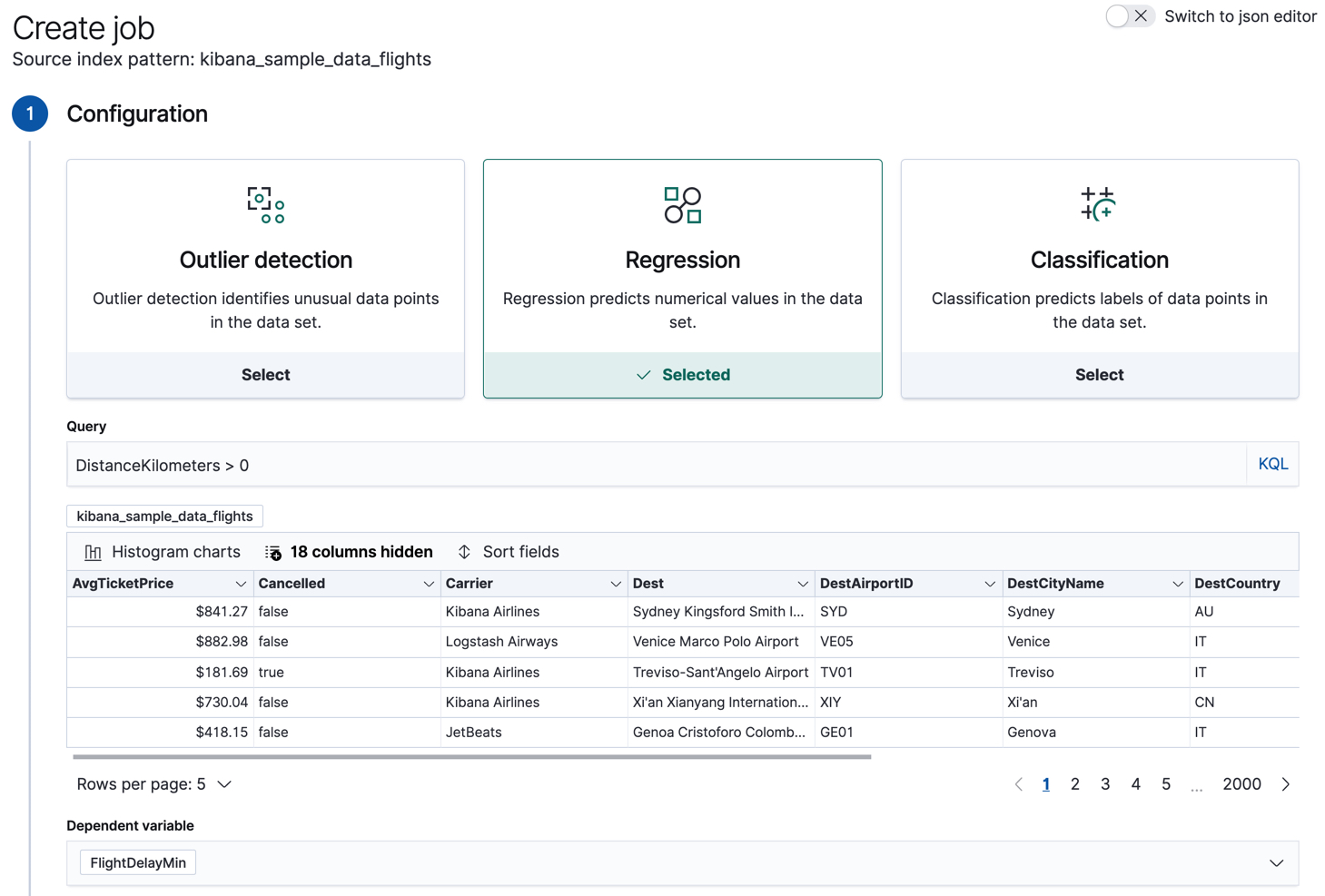
Choose
kibana_sample_data_flightsas the source index. -
Choose
regressionas the job type. - Optionally improve the quality of the analysis by adding a query that removes erroneous data. In this case, we omit flights with a distance of 0 kilometers or less.
-
Choose
FlightDelayMinas the dependent variable, which is the field that we want to predict. -
Add
Cancelled,FlightDelay, andFlightDelayTypeto the list of excluded fields. These fields will be excluded from the analysis. It is recommended to exclude fields that either contain erroneous data or describe thedependent_variable.The wizard includes a scatterplot matrix, which enables you to explore the relationships between the numeric fields. The color of each point is affected by the value of the dependent variable for that document, as shown in the legend. You can use this matrix to help you decide which fields to include or exclude from the analysis.
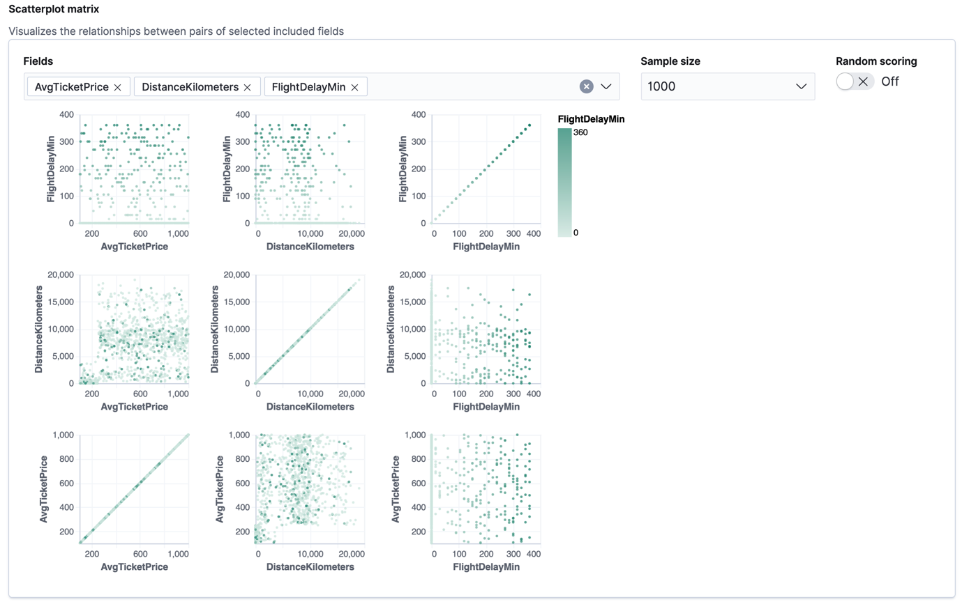
If you want these charts to represent data from a larger sample size or from a randomized selection of documents, you can change the default behavior. However, a larger sample size might slow down the performance of the matrix and a randomized selection might put more load on the cluster due to the more intensive query.
-
Choose a training percent of
90which means it randomly selects 90% of the source data for training. - If you want to experiment with feature importance, specify a value in the advanced configuration options. In this example, we choose to return a maximum of 5 feature importance values per document. This option affects the speed of the analysis, so by default it is disabled.
- Use a model memory limit of at least 50 MB. If the job requires more than this amount of memory, it fails to start. If the available memory on the node is limited, this setting makes it possible to prevent job execution.
-
Add a job ID (such as
model-flight-delay-regression) and optionally a job description. -
Add the name of the destination index that will contain the results of the analysis. In Kibana, the index name matches the job ID by default. It will contain a copy of the source index data where each document is annotated with the results. If the index does not exist, it will be created automatically.
API example
PUT _ml/data_frame/analytics/model-flight-delays-regression
{
  "source": {
    "index": [
      "kibana_sample_data_flights"
    ],
    "query": {
      "range": {
        "DistanceKilometers": {
          "gt": 0
        }
      }
    }
  },
  "dest": {
    "index": "model-flight-delays-regression"
  },
  "analysis": {
    "regression": {
      "dependent_variable": "FlightDelayMin",
      "training_percent": 90,
      "num_top_feature_importance_values": 5,
      "randomize_seed": 1000
    }
  },
  "model_memory_limit": "50mb",
  "analyzed_fields": {
    "includes": [],
    "excludes": [
      "Cancelled",
      "FlightDelay",
      "FlightDelayType"
    ]
  }
}
After you configured your job, the configuration details are automatically validated. If the checks are successful, you can proceed and start the job. A warning message is shown if the configuration is invalid. The message contains a suggestion to improve the configuration to be validated.
-
Choose
-
Start the job in Kibana or use the start data frame analytics jobs API.
The job takes a few minutes to run. Runtime depends on the local hardware and also on the number of documents and fields that are analyzed. The more fields and documents, the longer the job runs. It stops automatically when the analysis is complete.
API example
POST _ml/data_frame/analytics/model-flight-delays-regression/_start
-
Check the job stats to follow the progress in Kibana or use the get data frame analytics jobs statistics API.
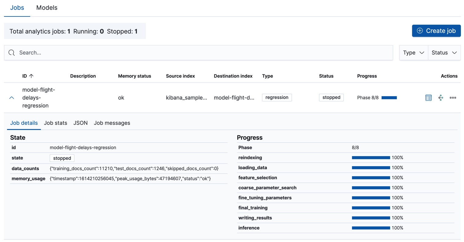
When the job stops, the results are ready to view and evaluate. To learn more about the job phases, see How data frame analytics jobs work.
API example
GET _ml/data_frame/analytics/model-flight-delays-regression/_stats
The API call returns the following response:
{
  "count" : 1,
  "data_frame_analytics" : [
    {
      "id" : "model-flight-delays-regression",
      "state" : "stopped",
      "progress" : [
        {
          "phase" : "reindexing",
          "progress_percent" : 100
        },
        {
          "phase" : "loading_data",
          "progress_percent" : 100
        },
        {
          "phase" : "feature_selection",
          "progress_percent" : 100
        },
        {
          "phase" : "coarse_parameter_search",
          "progress_percent" : 100
        },
        {
          "phase" : "fine_tuning_parameters",
          "progress_percent" : 100
        },
        {
          "phase" : "final_training",
          "progress_percent" : 100
        },
        {
          "phase" : "writing_results",
          "progress_percent" : 100
        },
        {
          "phase" : "inference",
          "progress_percent" : 100
        }
      ],
      "data_counts" : {
        "training_docs_count" : 11210,
        "test_docs_count" : 1246,
        "skipped_docs_count" : 0
      },
      "memory_usage" : {
        "timestamp" : 1599773614155,
        "peak_usage_bytes" : 50156565,
        "status" : "ok"
      },
      "analysis_stats" : {
        "regression_stats" : {
          "timestamp" : 1599773614155,
          "iteration" : 18,
          "hyperparameters" : {
            "alpha" : 19042.721566629778,
            "downsample_factor" : 0.911884068909842,
            "eta" : 0.02331774683318904,
            "eta_growth_rate_per_tree" : 1.0143154178910303,
            "feature_bag_fraction" : 0.5504020748926737,
            "gamma" : 53.373570122718846,
            "lambda" : 2.94058933878574,
            "max_attempts_to_add_tree" : 3,
            "max_optimization_rounds_per_hyperparameter" : 2,
            "max_trees" : 894,
            "num_folds" : 4,
            "num_splits_per_feature" : 75,
            "soft_tree_depth_limit" : 2.945317520946171,
            "soft_tree_depth_tolerance" : 0.13448633124842999
          },
          "timing_stats" : {
            "elapsed_time" : 302959,
            "iteration_time" : 13075
          },
          "validation_loss" : {
            "loss_type" : "mse"
          }
        }
      }
    }
  ]
}
Viewing regression results
editNow you have a new index that contains a copy of your source data with predictions for your dependent variable.
When you view the results in Kibana, it shows the contents of the destination index in a tabular format. It also provides information about the analysis details, model evaluation metrics, total feature importance values, and a scatterplot matrix. Let’s start by looking at the results table:
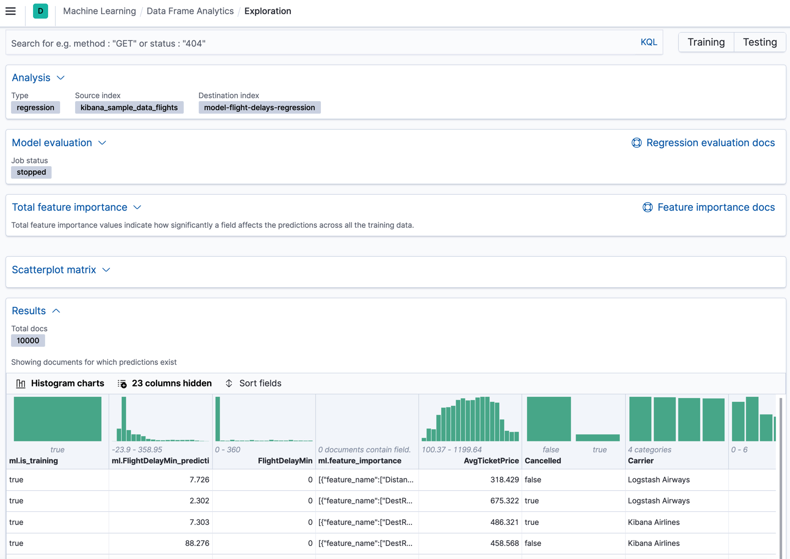
In this example, the table shows a column for the dependent variable (FlightDelayMin),
which contains the ground truth values that we are trying to predict. It also
shows a column for the prediction values (ml.FlightDelayMin_prediction) and a
column that indicates whether the document was used in the training set
(ml.is_training). You can filter the table to show only testing or training
data and you can select which fields are shown in the table. You can also enable
histogram charts to get a better understanding of the distribution of values in
your data.
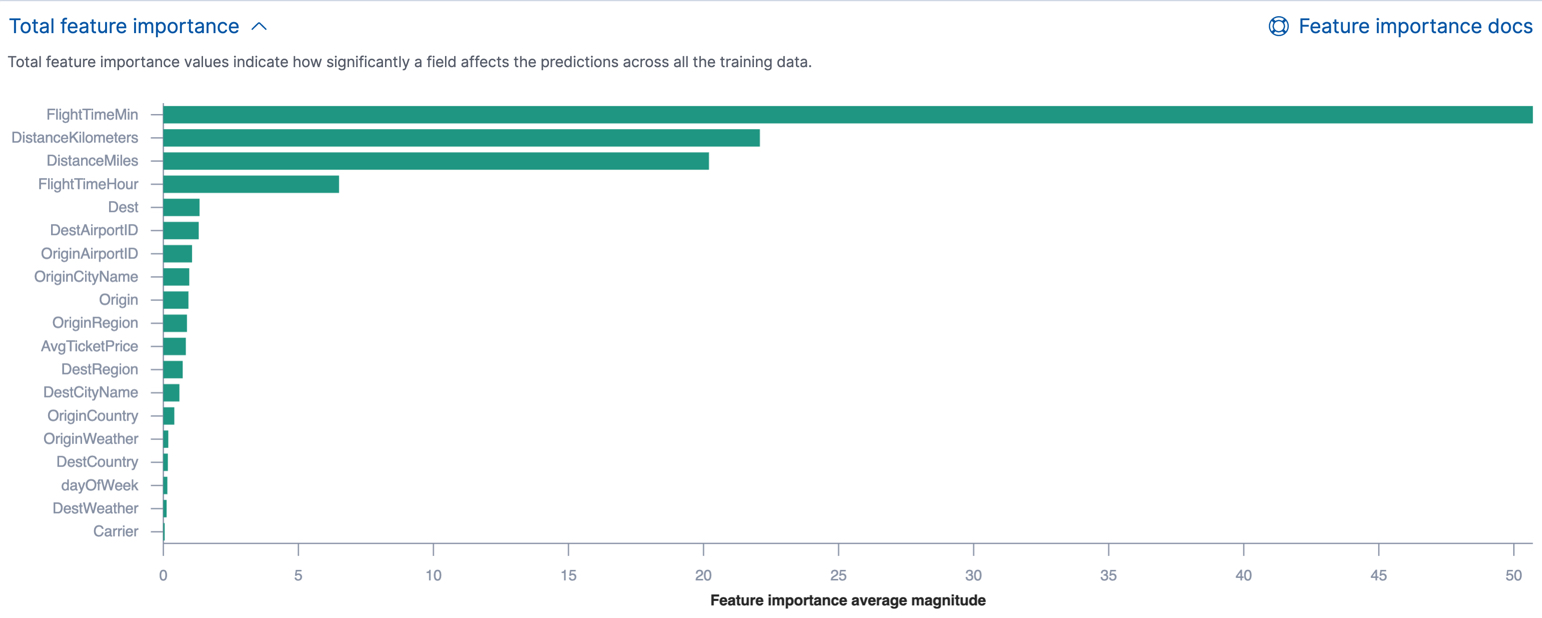
If you chose to calculate feature importance, the destination index also contains
ml.feature_importance objects. Every field that is included in the
regression analysis (known as a feature of the data point) is assigned a feature importance
value. This value has both a magnitude and a direction (positive or negative),
which indicates how each field affects a particular prediction. Only the most
significant values (in this case, the top 5) are stored in the index. However,
the trained model metadata also contains the average magnitude of the feature importance
values for each field across all the training data. You can view this
summarized information in Kibana:
You can also see the feature importance values for each individual prediction in the form of a decision plot:
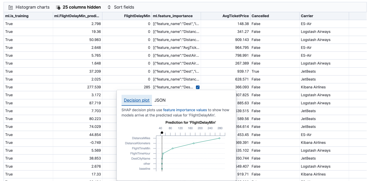
The decision path starts at a baseline, which is the average of the predictions for all the data points in the training data set. From there, the feature importance values are added to the decision path until it arrives at its final prediction. The features with the most significant positive or negative impact appear at the top. Thus in this example, the features related to the flight distance had the most significant influence on this particular predicted flight delay. This type of information can help you to understand how models arrive at their predictions. It can also indicate which aspects of your data set are most influential or least useful when you are training and tuning your model.
If you do not use Kibana, you can see summarized feature importance values by using the get trained model API and the individual values by searching the destination index.
API example
GET _ml/inference/model-flight-delays-regression*?include=total_feature_importance,feature_importance_baseline
The snippet below shows an example of the total feature importance details in the trained model metadata:
{
  "count" : 1,
  "trained_model_configs" : [
    {
      "model_id" : "model-flight-delays-regression-1601312043770",
      ...
      "metadata" : {
        ...
        "feature_importance_baseline" : {
          "baseline" : 47.43643652716527
        },
        "total_feature_importance" : [
          {
            "feature_name" : "dayOfWeek",
            "importance" : {
              "mean_magnitude" : 0.38674590521018903,
              "min" : -9.42823116446923,
              "max" : 8.707461689065173
            }
          },
          {
            "feature_name" : "OriginWeather",
            "importance" : {
            "mean_magnitude" : 0.18548393012368913,
            "min" : -9.079576266629092,
            "max" : 5.142479101907649
          }
          ...
|
The baseline for the feature importance decision path. It is the average of the prediction values across all the training data. |
|
|
The average of the absolute feature importance values for the |
|
|
The minimum feature importance value across all the training data for this field. |
|
|
The maximum feature importance value across all the training data for this field. |
To see the top feature importance values for each prediction, search the destination index. For example:
GET model-flight-delays-regression/_search
The snippet below shows a part of a document with the annotated results:
          ...
          "DestCountry" : "CH",
          "DestRegion" : "CH-ZH",
          "OriginAirportID" : "VIE",
          "DestCityName" : "Zurich",
          "ml": {
            "FlightDelayMin_prediction": 277.5392150878906,
            "feature_importance": [
            {
              "feature_name": "DestCityName",
              "importance": 0.6285966753441136
            },
            {
              "feature_name": "DistanceKilometers",
              "importance": 84.4982943868267
            },
            {
              "feature_name": "DistanceMiles",
              "importance": 103.90011847132116
            },
            {
              "feature_name": "FlightTimeHour",
              "importance": 3.7119156097309345
            },
            {
              "feature_name": "FlightTimeMin",
              "importance": 38.700587425831365
            }
            ],
            "is_training": true
          }
          ...
Lastly, Kibana provides a scatterplot matrix in the results. It has the same functionality as the matrix that you saw in the job wizard. Its purpose is to likewise help you visualize and explore the relationships between the numeric fields and the dependent variable in your data.
Evaluating regression results
editThough you can look at individual results and compare the predicted value
(ml.FlightDelayMin_prediction) to the actual value (FlightDelayMins), you
typically need to evaluate the success of the regression model as a whole.
Kibana provides training error metrics, which represent how well the model performed on the training data set. It also provides generalization error metrics, which represent how well the model performed on testing data.
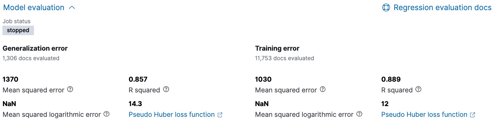
A mean squared error (MSE) of zero means that the models predicts the dependent variable with perfect accuracy. This is the ideal, but is typically not possible. Likewise, an R-squared value of 1 indicates that all of the variance in the dependent variable can be explained by the feature variables. Typically, you compare the MSE and R-squared values from multiple regression models to find the best balance or fit for your data.
For more information about the interpreting the evaluation metrics, see 6. Evaluate the result.
You can alternatively generate these metrics with the data frame analytics evaluate API.
API example
POST _ml/data_frame/_evaluate
{
 "index": "model-flight-delays-regression",
  "query": {
      "bool": {
        "filter": [{ "term":  { "ml.is_training": true } }]
      }
    },
 "evaluation": {
   "regression": {
     "actual_field": "FlightDelayMin",
     "predicted_field": "ml.FlightDelayMin_prediction",
     "metrics": {
       "r_squared": {},
       "mse": {},
       "msle": {},
       "huber": {}
     }
   }
 }
}
|
Calculates the training error by evaluating only the training data. |
|
|
The field that contains the actual (ground truth) value. |
|
|
The field that contains the predicted value. |
The API returns a response like this:
{
  "regression" : {
    "huber" : {
      "value" : 30.216037330465102
    },
    "mse" : {
      "value" : 2847.2211476422967
    },
    "msle" : {
      "value" : "NaN"
    },
    "r_squared" : {
      "value" : 0.6956530017255125
    }
  }
}
Next, we calculate the generalization error:
POST _ml/data_frame/_evaluate
{
 "index": "model-flight-delays-regression",
  "query": {
      "bool": {
        "filter": [{ "term":  { "ml.is_training": false } }]
      }
    },
 "evaluation": {
   "regression": {
     "actual_field": "FlightDelayMin",
     "predicted_field": "ml.FlightDelayMin_prediction",
     "metrics": {
       "r_squared": {},
       "mse": {},
       "msle": {},
       "huber": {}
     }
   }
 }
}
When you have trained a satisfactory model, you can deploy it to make predictions about new data.
If you don’t want to keep the data frame analytics job, you can delete it. For example, use Kibana or the delete data frame analytics job API. When you delete data frame analytics jobs in Kibana, you have the option to also remove the destination indices and data views.