Introduction to custom machine learning models and maps
How to use text-based datasets to build beautiful dashboards leveraging maps


 Share on Twitter
Share on Twitter

 Share on LinkedIn
Share on LinkedIn

 Share on Facebook
Share on Facebook

 Share by Email
Share by Email

 Print this page
Print
In Elasticsearch 8.0, we introduced the ability to run custom machine learning models, such as the ones based on BERT (Bidirectional Encoder Representations from Transformers), to perform natural language processing (NLP). This feature makes it easier to work with text-based datasets.
In this blog, I will put this concept into practice by showing how to extract location information from CNN articles and plot it on a map!
[Related article: How to use Elastic Maps to make public datasets observable]
Step 1. Gather the data
The first step is to gather a publicly available dataset. I have chosen the CNN dataset provided by Kaggle. You can download that and just import the CSV file as it is through Kibana, using the file upload feature inside machine learning.
Step 2. Import the machine learning model
The second step is to import the machine learning model that identifies categories like persons, locations, organisations, and miscellaneous. The models from Hugging Face work out of the box. Currently, there is no upload button inside Kibana for a machine learning model, so you’ll need to use your Eland client. To accomplish this, install the Eland client directly on your machine or check out the GitHub repository and run it as a Docker container.
If you want to use direct machine installation:
- Install it either by using pip python -m pip install eland or use the conda forge conda install -c conda-forge eland.
- That should be it; if you need more information, look at the GitHub repository of Eland.
If you want to use the docker container version:
- Clone the GitHub repository.
- Run the following commands to create a docker container from the repository. Don’t worry, this can take a few minutes to build: docker build -t elastic/eland.
- Start the container using an interactive mode: docker run -it --rm --network host elastic/eland.
- Now you are inside the container and can call any eland-related task!
Now that the Eland client is ready, you can import the model you need. Here, I’ll use our model provided by Elastic, available on Hugging Face. Before running the command below, adapt the --cloud-id to your correct one and use a user with the necessary permissions.
eland_import_hub_model \
--cloud-id home:...== \
-u elastic -p … \
--hub-model-id
elastic/distilbert-base-cased-finetuned-conll03-english \
--task-type ner \
--start
It will take a while to load the model and upload it to your cluster. While this happens, import one additional dataset and prepare an enrich policy!
Download this file and import it into your cluster using Kibana file upload. It contains the ISO codes, the continent, and the name. Now change to dev tools and use the following to create an enrich policy:
PUT /_enrich/policy/add2lettercodes
{
 "match": {
   "indices": "countries",
   "match_field": "name",
   "enrich_fields": ["alpha-2","region"]
 }
}First, create the enrich policy and clarify that it matches the name found in a document (e.g., Austria), with the name of the values in the countries. In this case, the document will get enriched with alpha-2: AT, region: Europe. An enrich policy needs to be executed before it is usable PUT _enrich/policy/add2lettercodes/_execute.
One last import, and you are all good to go. Use the continents view of ArcGis, download this as a shapefile, and use the file upload feature in maps.
Step 3. Adopt and modify the data
You have your model, and your data is in place. Ingest pipelines are needed to modify the data, so you can run the inference processor, send the document through the machine learning model, and analyse this. Open up dev tools and copy and paste the following:
PUT _ingest/pipeline/ml-models
{
   "processors": [
       {
           "inference": {
               "model_id": "distilbert-base-uncased-finetuned-sst-2-english",
               "target_field": "_ml-positiveornegative.ner",
               "field_map": {
                   "content": "text_field"
               }
           }
       },
       {
           "inference": {
               "model_id": "elastic__distilbert-base-cased-finetuned-conll03-english",
               "target_field": "_ml-distilbert.ner",
               "field_map": {
                   "content": "text_field"
               }
           }
       },
       {
           "script": {
               "lang": "painless",
               "if": "return (ctx['_ml-distilbert']['ner'].containsKey('entities'))",
               "source": "Map tags = new HashMap(); for (item in ctx['_ml-distilbert']['ner']['entities']) { if (!tags.containsKey(item.class_name)) tags[item.class_name] = new HashSet(); tags[item.class_name].add(item.entity);} ctx['tags'] = tags;"
           }
       },
       {
           "foreach": {
               "field": "_ml-distilbert.ner.entities",
               "ignore_failure": true,
               "processor": {
                   "enrich": {
                       "policy_name": "add2lettercodes",
                       "field": "_ingest._value.entity",
                       "target_field": "_temp.locations.convert.countries.{{_ingest._value.entity}}",
                       "ignore_failure": true
                   }
               }
           }
       },
       {
           "foreach": {
               "field": "_temp.locations.convert.countries",
               "ignore_failure": true,
               "processor": {
                   "append": {
                       "field": "locations.countries",
                       "value": "{{_ingest._value.alpha-2}}",
                       "ignore_failure": true
                   }
               }
           }
       },
       {
           "foreach": {
               "field": "_temp.locations.convert.countries",
               "ignore_failure": true,
               "processor": {
                   "append": {
                       "field": "locations.continents",
                       "value": "{{_ingest._value.region}}",
                       "ignore_failure": true
                   }
               }
           }
       },
       {
           "remove": {
               "field": "_temp.locations.convert",
               "ignore_failure": true
           }
       },
       {
           "set": {
               "field": "ingest_timestamp",
               "value": "{{_ingest.timestamp}}"
           }
       }
   ]
}This will create an ingest pipeline called ml-models. Lastly, you’ll need to perform a reindex. I called the original dataset that I imported through Kibana -data-orig. You will get a task id — copy that one, and use the GET _tasks/id call to see the progress.
POST _reindex?wait_for_completion=false
{
 "source": {
   "index": "cnn-data-orig",
   "size": 50
 },
 "dest": {
   "index": "cnn-data-ml",
   "pipeline": "ml-models"
 }
}The reindex is done. Take a look at an example document and the tags that are added:
{
   "tags": {
       "LOC": [
           "Allianz Arena Munich",
           "Macedonia",
           "Germany"
       ],
       "ORG": [
           "CNN",
           "Manchester City",
       ],
       "MISC": [
           "Germans",
           "World Cup",
           "German",
           "European"
       ],
       "PER": [
           "Timo Werner",
           "Igor Angelovski",
           "Leroy Sane",
           "Read MoreShortly",
           "Joachim Loew",
           "Gundogan"
       ]
   }
}That is a long list. In this case, we can see that we identified persons, locations, miscellaneous, and organisations.
Taking a closer look at the locations, we can identify that the model also recognises certain things like stadiums, like the Allianz Arena in Munich for soccer. However, Elasticsearch does not know where the Allianz Arena in Munich is. Watch out for an upcoming blog post on this topic using runtime field lookups!
Our enrichment runs over each of the elements inside LOC. So it added the ISO code for Macedonia and Germany, and the continent of Europe.
{
   "locations": {
       "countries": [
           "MK",
           "DE"
       ],
       "continents": [
           "Europe",
           "Europe"
       ]
   }
}So everything is done from a data preparation point. Let’s finally do some visualisations!
Step 4. Dashboarding and maps
You have completed all the necessary steps. Now, go ahead and combine all of it into a beautiful dashboard leveraging maps!
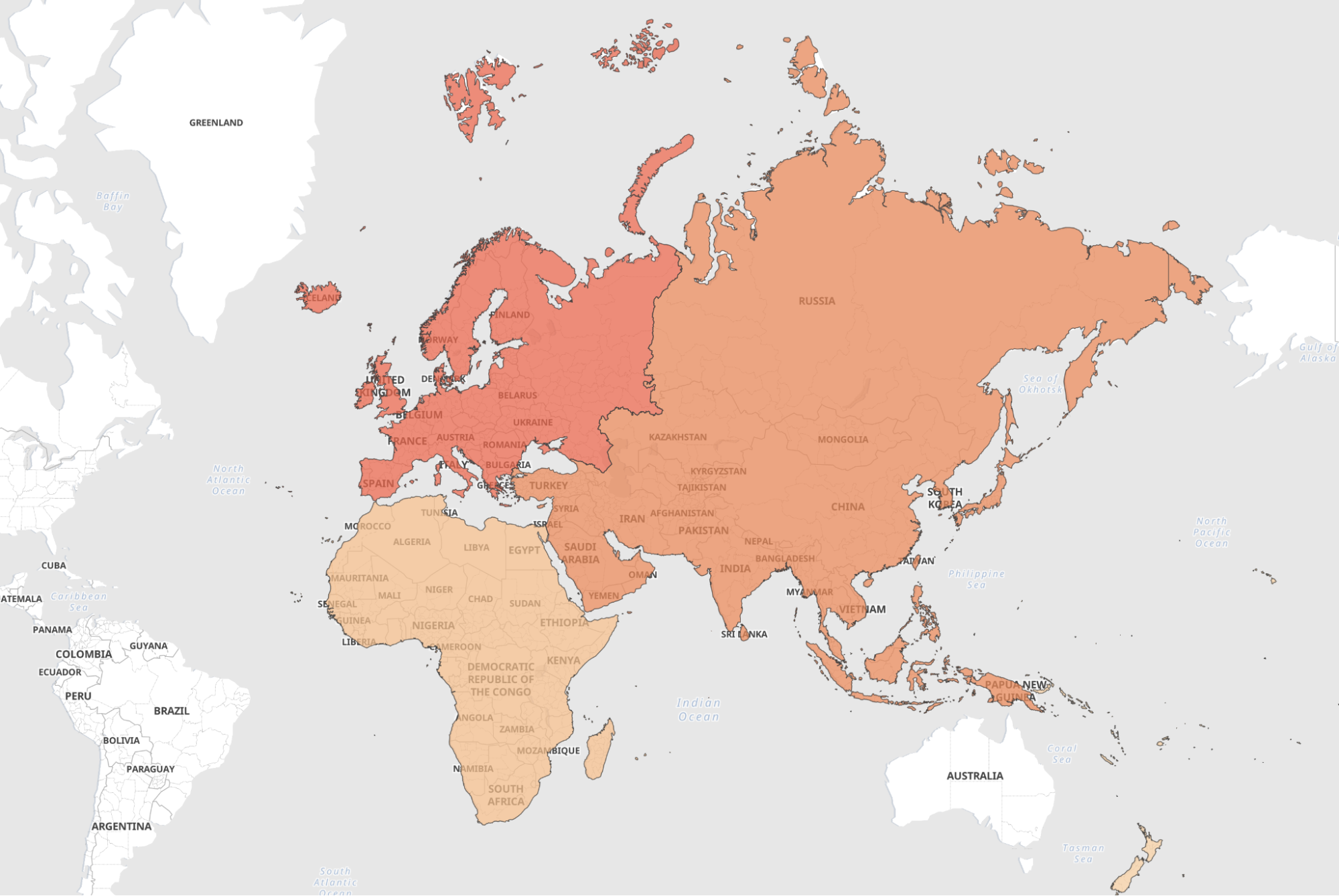
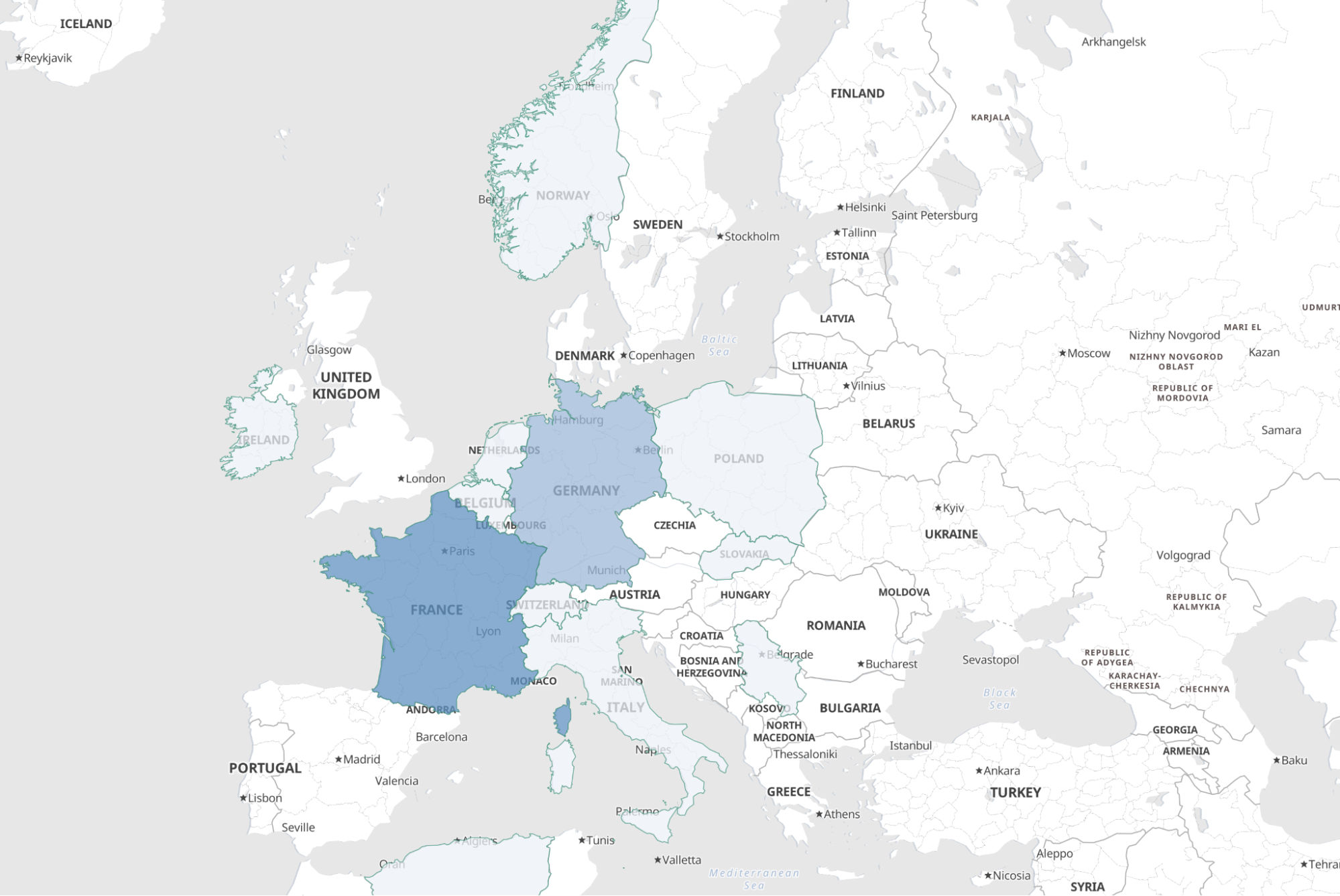
We are adding two layers: one for continents and one for countries. Setting both to different zoom levels, we can zoom into the world map and get from a continent to a country view. The colour shows how often a continent or country appears in an article.
Summary
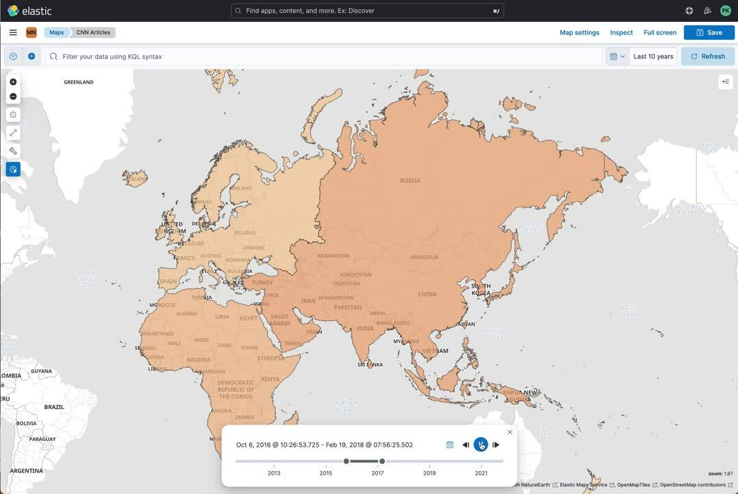
This very technical blog post covers many topics inside Elasticsearch and Kibana — uploading files, using ingest pipelines, enrich processors, and more! There is one last goodie I wanted to show you: the time slider in maps. We can now see how the news coverage has changed over time for a continent:
Share
- Share on Twitter
Share on Twitter
- Share on LinkedIn
Share on LinkedIn
- Share on Facebook
Share on Facebook
- Share by Email
Share by Email
- Print this page
Print