0.35% trained, 100% competitive: the frozen-tower architecture behind jina-embeddings-v5-omni
The latest jina embeddings model generates multimodal embeddings for text, images, video and audio, competing with models nearly 6x its size on vector search while training just 0.35% of the weights.
jina-embeddings-v5-omni is our latest multimodal embedding model. It generates embeddings for text, image, video, and audio. Among open-weight models that support those modalities, it’s the best-performing under 2 billion parameters. The notable part is how little of it we actually trained. Every encoder tower stayed frozen, and only about 0.35% of the model's weights (projectors and a handful of delimiter tokens) were ever updated during training. We call this architecture pattern Geometry-preserving Embeddings via Locked Aligned TOwers (GELATO). Let's break down each letter of this acronym:
Geometry-preserving Embeddings:
jina-embeddings-v5-omnisits atop the foundation laid byjina-embeddings-v5-text. That original text embedding space is completely unchanged, with its geometry left wholly intact.Locked: Synonymous with "frozen." All of the towers in this architecture have their weights locked.
Aligned: Aligning the other modalities with the text model's vector space, allowing for cross-modal comparison.
TOwers: Modality component that converts one type of raw input into vectors.
The model comes in two variants: small and nano. The former has more parameters (1.57 billion) than the latter (0.95 billion), but functionally their architectures are nearly identical. For the sake of brevity, we mostly focus on jina-embeddings-v5-omni-small in this article.
What are vectors, towers and frozen encoders?
jina-embeddings-v5-omni relies on three core machine learning (ML) concepts: vectors, towers, and frozen weights. Here's what each means; feel free to skip ahead if you're already familiar with them.
How vectors represent data in embedding models
How does AI understand abstract concepts? Can a machine comprehend what "ice cream" is? Does it understand that "chocolate fudge" and "rocky road" have more in common with each other than "sorbet"? The answer, surprisingly, is yes. The mechanism that makes it possible is the vector.
Take a look at this diagram.
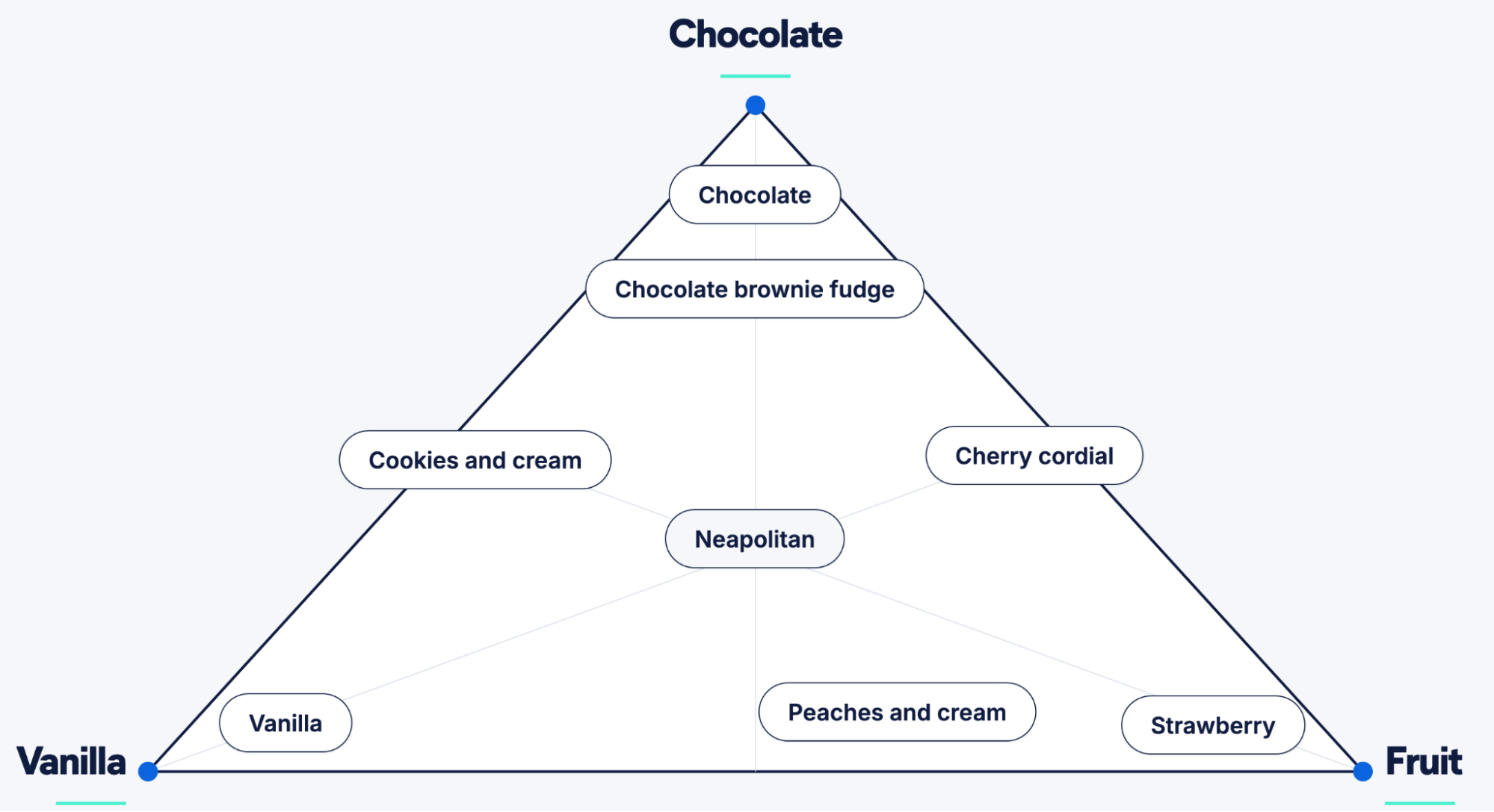
If you tried visualizing a way to organize all ice cream flavors, you may end up with something like this: a simplex (triangle) with three vertices, each representing a base flavor. Each flavor is closer to or farther from each vertex, depending on how much of the corresponding base makes up that particular flavor. Chocolate ice cream is all chocolate, so it hugs the top vertex. Vanilla has a similar affinity for the bottom-left vertex. But cookies and cream is roughly a 50/50 mix, so it's about equidistant from both. Neapolitan blends all three, so it sits at the center of the triangle.
This is functionally how vectors work. These flavors get funneled into an ML model (more specifically known as an embedding model) that will then generate coordinates for each of these flavors along this simplex. By measuring the distance between coordinates, software can parse how related or unrelated two flavors are. It's easy to see that "chocolate" and "chocolate brownie fudge" are closely related flavors because they sit close to one another, but "strawberry" and "cookies and cream" are far away from each other, so we can infer that they aren’t similar.
It won't be quite this simple though. Rather than three labeled points, real embeddings run along hundreds or even thousands of dimensions. Nor will they have nice, human-readable labels; the vertex markers are something that only the model understands. The benefit, though, is that we can graph basically anything like this.
To clarify some jargon: These coordinates = vectors = embeddings. For the rest of this article, we use these terms interchangeably.
Much like how embeddings go by many different names, so too do the models that create them.
What is a tower in multimodal embedding models?
The term tower comes from Contrastive Language-Image Pre-training (CLIP), a model released by OpenAI in 2021 that was one of the first to learn a shared embedding space across text and images. In CLIP, each modality is handled by a completely separate model. On an architecture schematic, these models look like towers standing side by side, each taking one type of input and producing vectors in a shared space. The name stuck, and you'll see it used broadly across multimodal ML.
In the context of jina-embeddings-v5-omni, the word is used a bit more loosely. Its architecture doesn't have true parallel towers in the CLIP sense. All modalities ultimately funnel into a single central text model, rather than sitting as equals beside it.
With that caveat in place: A tower (or modality component) is a pipeline that converts one type of raw input into vectors. A text tower vectorizes strings, and a vision tower generates image embeddings. An audio tower does the same for sound.
Why freeze a tower instead of training it?
If we want multimodal capabilities, could we Frankenstein multiple towers that handle each of those inputs together into one model? The issue with this approach is that vectors from different models aren’t intelligible to each other. Images will exist in one vector space and audio in another, for example. This means that we have no ability to compare across different modalities. Think of the vectors outputted from one model as existing in their own language. Let's say our audio tower outputs Spanish and our image tower outputs English. Conceptually, the vectors can be describing the same things, but downstream tools that try to make use of these embeddings are "monolingual," so we're out of luck.
The CLIP-style approach is to take several towers and train them together, letting them all reshape each other until their outputs agree. It's sort of like having Spanish and English speakers try to communicate for long enough that they eventually all start speaking Spanglish.
This approach works, but it has a side effect: Towers that you already had working get remodeled in the process. Any embeddings that they produced before are now incompatible with any that are produced by the older version of the tower. If you had a text tower and generated 100 million embeddings with it, you would now need to re-embed all of those strings.
To combat this issue, you can freeze certain towers. This locks their weights, which are the knobs and dials that influence how they behave. This way, training never changes them. What you train instead is a small projector that translates one tower's output into another tower's language. Many different models train some portion of projectors and towers while leaving some others frozen. What makes jina-embeddings-v5-omniunique is that we froze every encoder and trained only the projectors and delimiter tokens. By the end of this article, you’ll understand exactly how that works.
You can think of these frozen and trainable components as clusters of neurons or isolated regions of the mind, and the whole embedding model (jina-embeddings-v5-omni) as the entire brain. Between these learning-capable components sit fixed math operations, such as merging, squashing, selecting, and rescaling numbers on their way from one tower to the next. They have no weights, so there’s nothing in them to freeze or train.
With that groundwork laid, here’s the full architecture.
How the jina embeddings multimodal architecture works
The architecture routes all modalities through frozen encoders and small trainable projectors into a single shared text embedding space.
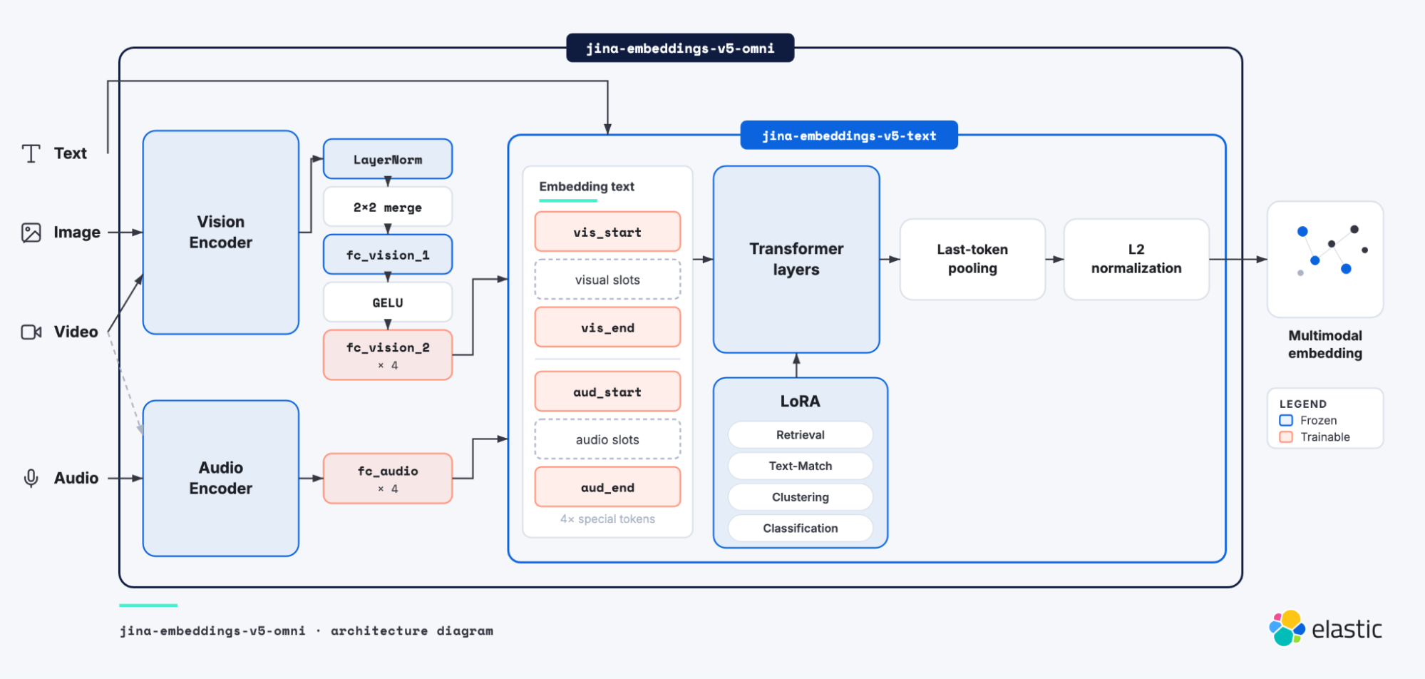
Why the text tower is the backbone
The first thing to notice here is the general flow of data in this diagram. Image, video, and audio inputs all (eventually) end up in the same space as text inputs. Why is the architecture set up like this?
jina-embeddings-v5-omni builds on top of jina-embeddings-v5-text: It retains its text-processing backbone and extends it with pretrained vision and audio components.
This has two main advantages:
The text model is already state of the art for its size and what it does, and it stays completely untouched. There’s no need to fix what isn't broken. We also don't need to re-embed anything we already embedded with
jina-embeddings-v5-text.A single shared vector space is what makes cross-modal search work at all. Because image, audio, and text all resolve to vectors in the same geometry, you can query an image with text, or audio with text, and compare them directly with cosine similarity (a similarity measure based on the angle between two vectors). If each modality lived in its own separate space, those comparisons would be meaningless.
How vision and audio encoders feed into the text model
The first step in building upon the foundation set by jina-embeddings-v5-text is integrating vision and audio encoders into this architecture. In this case, we use the existing Qwen3.5 vision encoders and the Qwen2.5-Omni audio encoder, which themselves have been adapted from SigLIP2 and Whisper-large-v3, respectively. They’re ultimately what’s responsible for generating raw vectors for all vision- and audio-based data. The emphasis is on raw here, since much transformation still needs to be done afterward.
How the vision encoder processes images
In the case of images, we’re borrowing more from Qwen than just the encoder. Additional plumbing inherited from Qwen is attached to the output of the encoder. Let's walk through what comes out of the encoder and how the inherited downstream components transform that output.
Vision encoder (frozen)
Let's use an image as our primary example, since the visual component of video is basically identical. Take this image of a banana split.
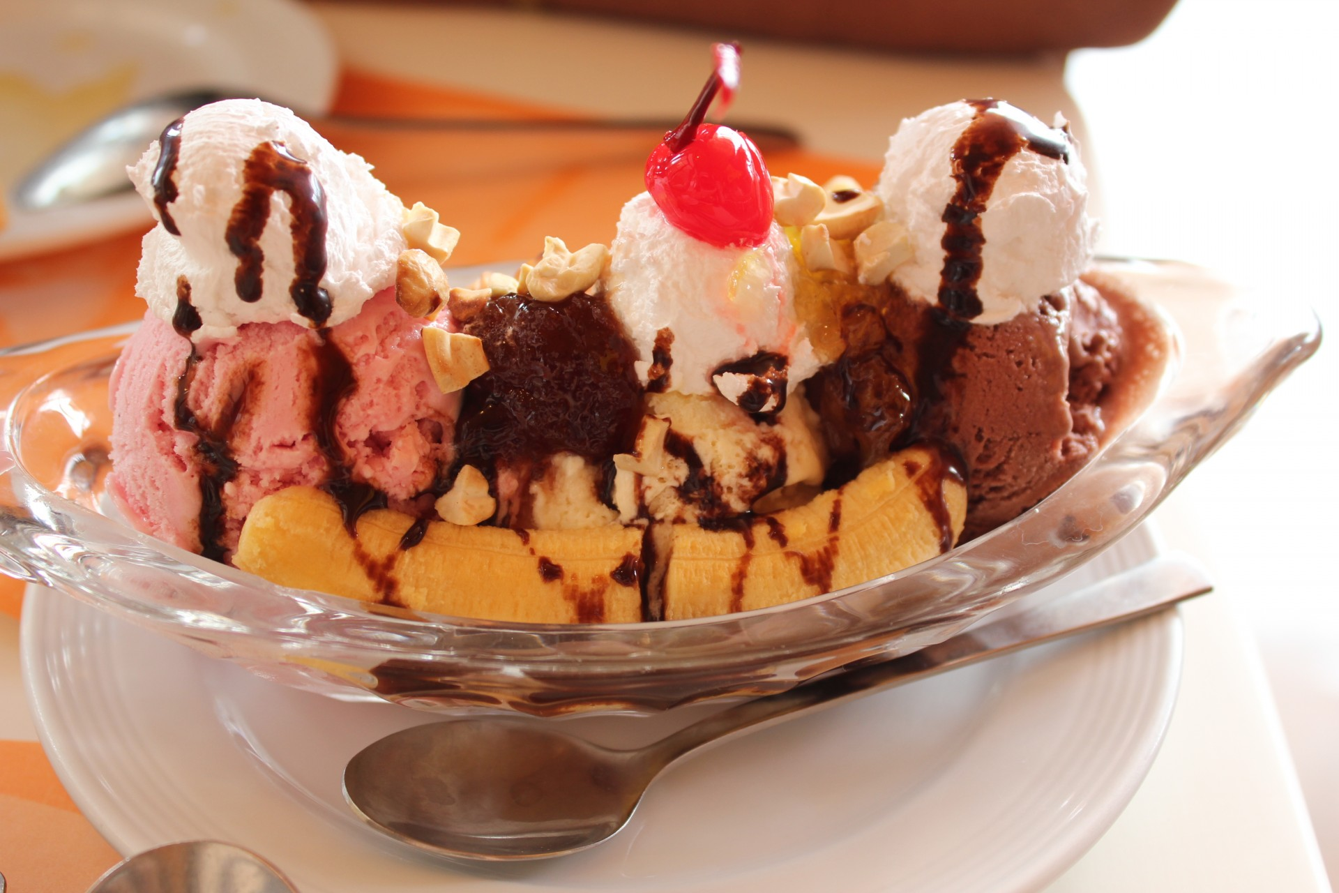
Rather than generating one single, clean vector embedding for this image, the vision encoder breaks the image up into 14-pixel by 14-pixel sections and generates a tiny patch token (basically a mini-vector) for each of these sections.
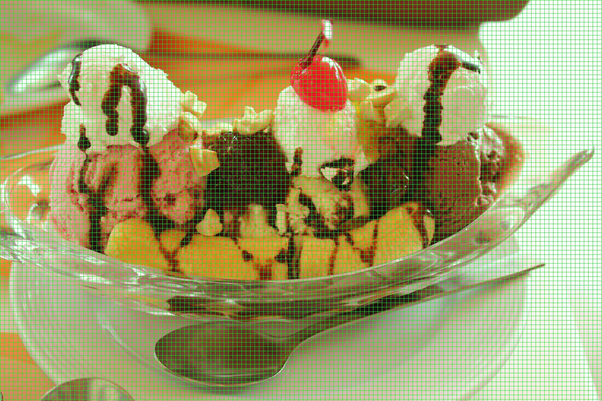
While still inside of the vision encoder, each token looks at every other token that makes up the image and pulls in information from the ones relevant to it, updating its own vector based on that context. This process allows us to preserve fine-grained details. Now, instead of one single vector for the whole image, we have multiple, smaller vectors that represent particulars of the whole dish.
LayerNorm (frozen)
LayerNorm rescales each patch's numbers so they sit in a consistent range before anything else touches them. It stops some patches from being wildly larger than others and drowning out the rest.
2x2 merge
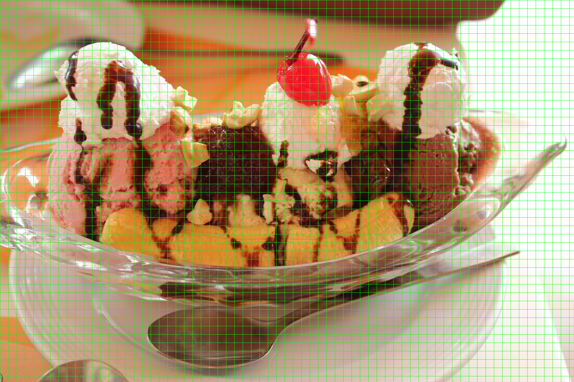
We saw in the vision encoder section that we split up the image into small, 14-pixel by 14-pixel squares. However, processing this many patch tokens will become expensive downstream. For this reason, the 2x2 merge operation consolidates four patch tokens into one. The squares are now 28 pixels by 28 pixels. The corresponding patch tokens are similarly consolidated.
fc_vision_1 (frozen)
fc_vision_1 is the first of two matrix multiplies; it mixes the merged patch numbers into a new set. This layer is inherited from Qwen and left as is.
GELU
Gaussian Error Linear Unit (GELU) is a gate applied to each number. It lets useful signals through and squashes the rest toward zero. It’s the one nonlinear step and is ultimately what lets the two fc_vision layers together learn shapes that a single flat multiply couldn't.
fc_vision_2 (trainable)
As mentioned earlier, trying to put Qwen image embeddings directly into the same vector space as Jina text embeddings would be like trying to include a Spanish sentence in an English novel. Outside of its native context, its meaning is totally lost.
That is what the trainable projector fc_vision_2 is here to fix. It learns to translate the image embedding into something that jina-embeddings-v5-text can understand. For this reason, you can think of a trainable projector as a translator.
The emphasis belongs on trainable: This is the first component we’ve encountered in our walkthrough so far that isn’t frozen. Many components of this architecture are frozen, meaning that their weights are locked and never change during training, but fc_vision_2 is one of the few parts that actually gets updated, because it has to learn how to translate Qwen's image dimensions into a form that lands meaningfully inside Jina's text space.
× 4
By now, you may have noticed that fc_vision_2 has a "× 4" marked on the bottom, along with fc_audio, both encoders, and the ″Embedding text″ section within jina-embeddings-v5-text. In this case, it represents four different instances of fc_vision_2, each optimized and tuned to one of four slightly different tasks, outlined below.
Task | What it facilitates | Example user input | Example end result | Note |
|---|---|---|---|---|
Retrieval | Finds a similar match for the input (that is, standard Google search) | "melting ice cream" as a string/text | Picture of a fallen ice cream cone on asphalt |
|
Text-matching | Judges how similar inputs are | A text string "melting ice cream" and an image of a fallen ice cream cone on asphalt | Score judging how similar the two inputs are | The name of this task is a bit of a misnomer. It's called text-matching, but it works for any modality, not only text. |
Clustering | Groups data into clusters | A large array of ice cream images | Lets the user discover natural groups, like "sundaes" and "popsicles" |
|
Classification | Places data into predefined buckets | Two string labels: "melting" and "intact", along with a large array of ice cream images | Sorts the array of ice cream images into the two provided categories, based on their proximity in vector space to the label embeddings |
|
To clarify, the "Example end result" column is the takeaway after some additional math and processing happens once the output vector is generated. The point is that jina-embeddings-v5-omni only generates vectors. Those vectors take on a mildly different form to optimize for the selected task type.
These task types are also explicitly outlined in the Low-Rank Adaptation (LoRA) component of the architecture diagram, which we'll cover in a moment.
How the audio encoder processes sound
Before we go any deeper into the trenches of our model architecture, let's back up and see how the audio-oriented path differs and how it stays the same. If you were able to follow along during the vision section, the audio portion will be a breeze. We have no extra inherited plumbing from Qwen this time, only the audio encoder and one trainable projector.
Audio encoder (frozen)
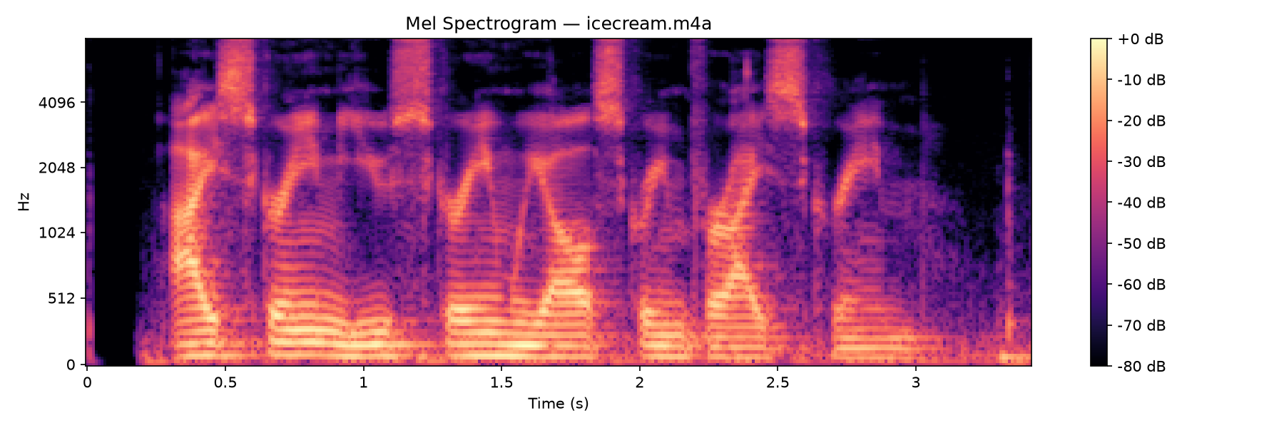
Before audio can enter the encoder, it needs to be converted into a form that the encoder can work with. Raw audio is a one-dimensional wave, which isn't particularly useful to a neural network on its own. Instead, the audio is first transformed into a mel spectrogram: a 2D representation that maps frequency against time, weighted to emphasize the frequency ranges that the human ear is most sensitive to. Think of it as a visual fingerprint of the sound. Below is a mel spectrogram of a person saying, "I scream, you scream, we all scream for ice cream."
That spectrogram is then sliced into fixed-length 40ms chunks, analogous to how the vision encoder breaks an image into 14×14 pixel-tiles. The encoder then produces one token per chunk.
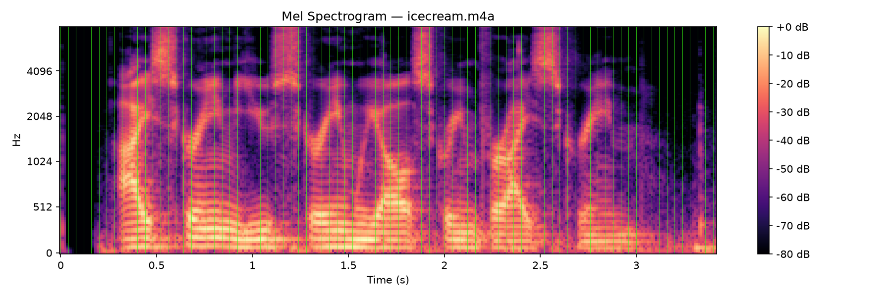
This matters for the same reason it does in the vision pipeline: Fine-grained detail would otherwise be lost. A single embedding for the full phrase "I scream, you scream, we all scream for ice cream" would smear everything into one blurry vector. Slicing it into short chunks keeps each fragment of sound intact, so the model can later distinguish "scream" from "cream" rather than collapsing them into an average. The same applies to music, animal noises, environmental sounds, and more.
fc_audio (trainable)
Once the encoder has produced its tokens, fc_audio performs the same translation role that fc_vision_2 does for images: It projects each audio token from the encoder's 1280-dimensional output space into jina-embeddings-v5-text’s hidden dimension (1024 for small, 768 for nano). Like fc_vision_2, it carries a "× 4" in the architecture diagram, meaning that there are four instances, each optimized for a specific task type (retrieval, text-matching, clustering, and classification).
Delimiters (trainable)
We need to convey to jina-embeddings-v5-text that this embedding represents an unexpected modality. We can do this pretty easily with delimiters. In the world of HTML, this looks like:
<p> Your text here </p>The first and last <p> tag conveys that everything in between them is a paragraph element.
In our case, things are a bit more complicated. For audio, the architecture diagram shows the delimiters as <aud_start> and <aud_end>, but that isn't quite accurate. The delimiters themselves are actually vectors rather than hard-coded strings.
Each task type has its own pair of delimiter vectors (hence the "4 × special tokens"). These vectors are identical every time rather than being different for each audio embedding. So a task type of retrieval with an audio input type always gets start delimiter vector X and end delimiter vector Y; text-match with audio input always gets a start delimiter vector A and an end delimiter vector B, and so on.
This is necessary because the Transformer layers component only understands vectors. So, by the time the audio embedding makes its way there, it looks like:
<aud_start_vector_delimiter>
<aud_patch_token_1>
<aud_patch_token_2>
<aud_patch_token_3>
...
<aud_end_vector_delimiter>
The same pattern applies to images:
<vis_start_vector_delimiter>
<vis_patch_token_1>
<vis_patch_token_2>
<vis_patch_token_3>
...
<vis_end_vector_delimiter>
Video is where this gets interesting. Up to 32 evenly spaced-out frames are pulled from the video and fed into the vision encoder.
Rather than producing one delimiter-wrapped segment, each sampled frame gets its own <vis_start> / <vis_end> wrapper, and these per-frame segments are concatenated into one long sequence:
<vis_start> [frame 1 patch tokens] <vis_end>
<vis_start> [frame 2 patch tokens] <vis_end>
...
<vis_start> [frame 32 patch tokens] <vis_end>
This is what makes multi-frame video work: Rather than averaging frames or treating them separately, the transformer receives the whole video as one token stream, allowing its attention to relate tokens across frames. This means that earlier frames can inform how later ones are interpreted. If the video does have an audio component, it's pulled out and fed into the audio encoder and ultimately prepended to the frame sequence.
<aud_start> [audio patch tokens] <aud_end>
<vis_start> [frame 1 patch tokens] <vis_end>
<vis_start> [frame 2 patch tokens] <vis_end>
...
The transformer layers component then processes this entire concatenated sequence as a single input.
Jina text transformer layers (frozen)
We’ve generated patch tokens for our images, videos, and audio files. We’ve also wrapped them inside of vector delimiters, all for the sake of having them understood by these layers. They’ll allow each patch token to examine the other patch tokens and determine whether they need to update themselves based on the surrounding context. I know what you're thinking:
Didn't we already do this inside of the encoder? We split up the image into 14-pixel by 14-pixel sections and generated patch tokens for each section, and then the encoder updated each patch token based on surrounding context within the same image.
And you're right! We did. But there's a key difference now.
Originally, that recontextualization ran on the attention of Qwen's vision encoder. The operation within the Transformer layers runs the frozen Jina text transformer's attention. It’s the same operation with different learned parameters, so it transforms the tokens differently.
Think of it like a move: The projector is the flight and the moving trucks. It physically relocates you from vision land to text land, landing you in the right city and even the right neighborhood. The transformer's attention is what happens after you've unpacked. You're already home; you spend the next few weeks figuring out exactly where you fit, meeting the neighbors, finding your bearings, and adjusting your exact spot based on who's actually around you. You did the macro move already. This is the micro fine-tuning.
Lastly, the <vis_end_vector_delimiter> will absorb all the information from the patch tokens it wraps.
LoRA (frozen)
LoRA is a way of fine-tuning an existing model without completely retraining it. It’s a small set of extra adjustment knobs bolted onto the transformer that nudges its behavior to optimize for one of the specific tasks (such as retrieval or classification).
Last-token pooling
Since <vis_end_vector_delimiter> absorbed all the other patch tokens into itself, we don't need to consider anything except it, so we throw the rest away. It acts as a stand-alone embedding that represents a summary of the whole.
L2 normalization
<vis_end_vector_delimiter> could be any length now, which is no good. This step shrinks or stretches it so its length is exactly 1, without changing the direction it points. This is tidying so that comparing it to other vectors later is a fair, clean angle comparison. It changes only the vector’s scale, not what it means.
Enough about ice cream
As we've journeyed our way through jina-embeddings-v5-omni, we’ve been careful to outline which components are frozen and which ones are trainable. By now, you may have noticed that every single tower has been frozen. In fact, only the small projectors (translators) and delimiter tokens have been trainable. We dubbed this architecture pattern GELATO. This makes the entire training process significantly cheaper.
To be clear, we didn't invent the concept of frozen towers. Prior work on Locked-image Tuning (LiT), VISTA, and Multi-modAl Retrieval model via Visual modulE pLugin (MARVEL) froze one side or the other. What no one had done before GELATO was push the idea to its limit: text, image, video, and audio all in one model with every encoder frozen. The only trained pieces are a single projector layer per modality and a handful of delimiter tokens.
But is it any good?
Benchmark results: jina embeddings vs. other multimodal embedding models
There's no point in building out a model and releasing it if you don't even know if it's any good, especially compared to the competition. That's why we have benchmarks and evaluation frameworks. The benchmarks that jina-embeddings-v5-omni was run against are Massive Image Embedding Benchmark (MIEB), Massive Audio Embedding Benchmark (MAEB), Massive Multimodal Embedding Benchmark–Video (MMEB-Video), and Massive Multilingual Text Embedding Benchmark (MMTEB).
As for the models we compare against, it's important not to make apples and oranges comparisons. For that reason, we’re specifically using open-weight omni-style models with support for the same media types:
Evaluation

The table above is sorted by parameter count. Models with the fewest parameters are clustered at the top, and models with the most parameters hug the bottom. This context is important because performance alone isn't the final variable. If a $100 ice cream with gold flakes and the finest dairy milk tastes the same as (or worse than) the average gallon of ice cream that you can buy from your local grocery store, it would be silly to buy it, because you're paying a massive premium for nothing.
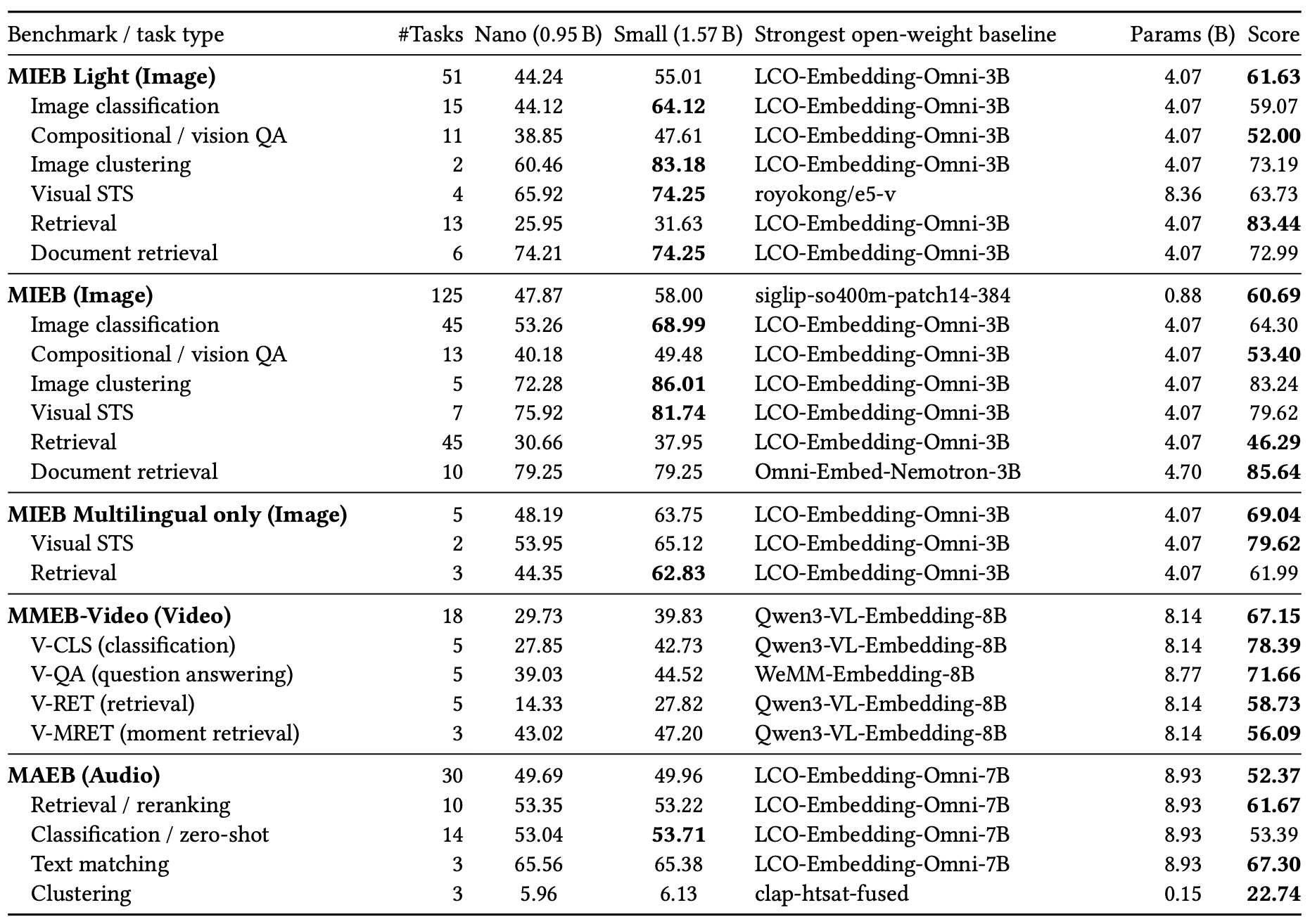
A similar situation is unfolding here. jina-embeddings-v5-omni-small and nano outperform every other model on text, despite ranking low to middle in terms of parameter count.
Audio performance is strong, as well. jina-embeddings-v5-omni-small and nano beat out all other models except those from LCO, which they both trail by about 2 to 3 points.
The gap shrinks when considering image performance, particularly with jina-embeddings-v5-omni-small. It beats both LanguageBind and Omni-Embed-Nemotron-3B. It lags less than a point behind both LCO models, despite the fact that they have 4.70 billion and 8.93 billion, respectively, compared to Jina’s 1.57 billion.
Video is the weakest performer for our models, though even in that case jina-embeddings-v5-omni-small still beats Omni-Embed-Nemotron-3B, which has three times as many parameters. Ultimately, when these scores are averaged out, you get the following rankings:
Model | Number of parameters (B) | Average score |
|---|---|---|
| 8.93 | 54.43 |
| 1.57 | 54.04 |
| 4.70 | 53.83 |
| 0.95 | 47.49 |
| 4.70 | 41.21 |
| 1.14 | 35.82 |
LCO-Embedding-Omni-7B has nearly six times the number of parameters as jina-embeddings-v5-omni-small but barely squeaks past it in average performance.
One benchmark deserves a special callout for anyone building search or retrieval augmented generation (RAG): visual document retrieval, measured on the ViDoRe benchmark.
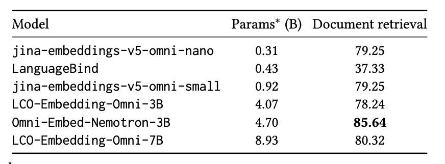
Here, jina-embeddings-v5-omni-small scores 79.25 using only 0.92 billion active text-and-image parameters, ahead of LCO-Embedding-Omni-3B (78.24) and within striking distance of LCO-Embedding-Omni-7B (80.32), a model nearly 10 times its size on that path. nano matches that exact same 79.25 score with just 0.31 billion active parameters. The larger Omni-Embed-Nemotron-3B does take the top spot at 85.64, but it carries roughly five times the active parameters of jina-embeddings-v5-omni-small, so our models remain the most parameter-efficient of the group. If your workload is retrieving pages of documents by their layout and text, this is the number to weigh.
Limitations of frozen-tower multimodal embeddings
GELATO's frozen-tower design delivers strong results at low training cost, but it comes with trade-offs worth naming plainly. As already mentioned, the most consistent weak spot is video. jina-embeddings-v5-omni-small trails the LCO models on video, and moment retrieval (locating a specific event within a clip) is the weakest subtask of all. This is partly structural, since each frame produces its own token set before everything is concatenated and pooled into a single final embedding. Packing that much information into one embedding means that the early dimensions carry a heavier load, so video embeddings degrade faster than image embeddings when truncated to smaller sizes.
Audio has its own gap. While retrieval and classification scores are competitive, audio clustering is the weakest audio subtask (6.13 for jina-embeddings-v5-omni-small).
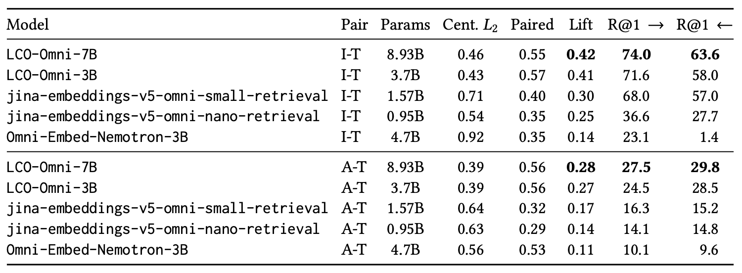
Cross-modal audio–text retrieval trails LCO-Omni-7B by 11–15 percentage points, a larger gap than the 6–7 points seen on the image–text (I-T) pair. The fc_audio projector is the natural next target for additional trainable parameters, suggesting the audio–text (A-T) alignment path has more room to grow than the multilayer vision pipeline.
How multimodal embeddings distribute in vector space
We've already discussed performance via benchmarks, but what about how the actual embeddings are distributed in vector space? How does that tangibly differ from model to model?
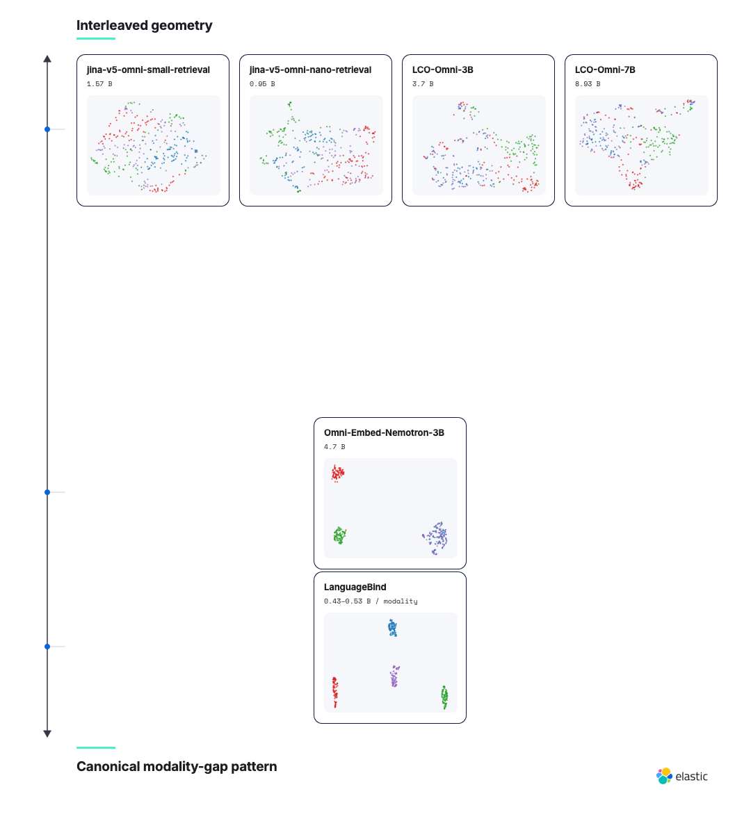
In the above illustration, data from video clips is funneled into each model and graphed in vector space. It’s then compressed down to two dimensions via the Uniform Manifold Approximation and Projection (UMAP) method for easy visualization. Each modality corresponds to a different component of the video:
Modality | Component of the video |
|---|---|
Image | Frame from the middle of the video |
Video | The full video |
Audio | Audio track from the video |
Text | Description of the video |
Immediately, some interesting patterns stand out.
Our models and the LCO models seem to have different modalities all mixed together, while LanguageBind and Omni-Embed-Nemotron-3B seem to lean more toward having their embeddings separated by modality.
Our models and the LCO models exhibit interleaved geometry for these vectors. This means that different modalities aren't clearly separated in vector space, but instead intermingle in similar areas. This is less pronounced with Omni-Embed-Nemotron-3B, since only image and video seem to occupy a similar space.
LanguageBind is fully separated, with different modalities occupying entirely different spaces. This is known as the modality-gap pattern.
So which one is better? In practice, interleaved geometry tends to be the more useful of the two, and it’s worth noticing that the strongest models in our benchmarks (ours and LCO's) all exhibit it. However, there are trade-offs.
Interleaved geometry excels at cross-modal retrieval, since everything is jumbled up together in the vector space and, therefore, much closer. It's easier to find a matching picture for the text "strawberry ice cream" when the text and image embeddings sit so close together in vector space.
When you're trying to do a same-modality task though, the image that was so conveniently within reach is now in the way. However, in practice, this is easily mitigated by metadata filtering on something like a “modality” field.
No such workaround exists for the issues inherent to models that exhibit the modality-gap pattern. It’s easy to find another video of syrup poured on ice cream, since all the videos are sitting together in isolation. But having modalities confined into clusters like that makes finding an accompanying image much harder.
Why this architecture?
GELATO gives a lot of performance for very little training. You keep all your towers as they are and train only small projectors and delimiter tokens, which is significantly cheaper than the alternatives. To put concrete numbers on "cheaper": for jina-embeddings-v5-omni-small, training just the vision projector updates 4.20 million parameters instead of the 920.6 million a full fine-tune would touch. At the same 15,000-step budget, that projector-only run finishes about 1.8 times faster and peaks at 7.52 GiB of GPU memory instead of 12.96 GiB. The audio path shows an even wider gap, with projector-only training running 3.2 to 3.9 times faster than full training. But how did we conclude this was the way to go? We used a process known as ablation.
Ablation is when you remove or change one piece of a system to see how much it actually mattered. Imagine you've been working on an ice cream recipe. Every time you make a tweak, like doubling the milk, swapping brown sugar for white, using vanilla beans instead of extract, or taking out the chocolate chunks, that's ablation.
Ablation in ML functions much in the same way. It asks whether removing, rearranging, freezing, or unfreezing certain components makes the whole system more, less, or equally as performant. In this case, we’re particularly interested in whether unfreezing certain components, and in what order, may affect performance. We conducted five ablation studies on the Qwen3.5 vision stack. The results are measured in mean nDCG@10 (normalized Discounted Cumulative Gain), a standard score for ranking quality where higher is better.
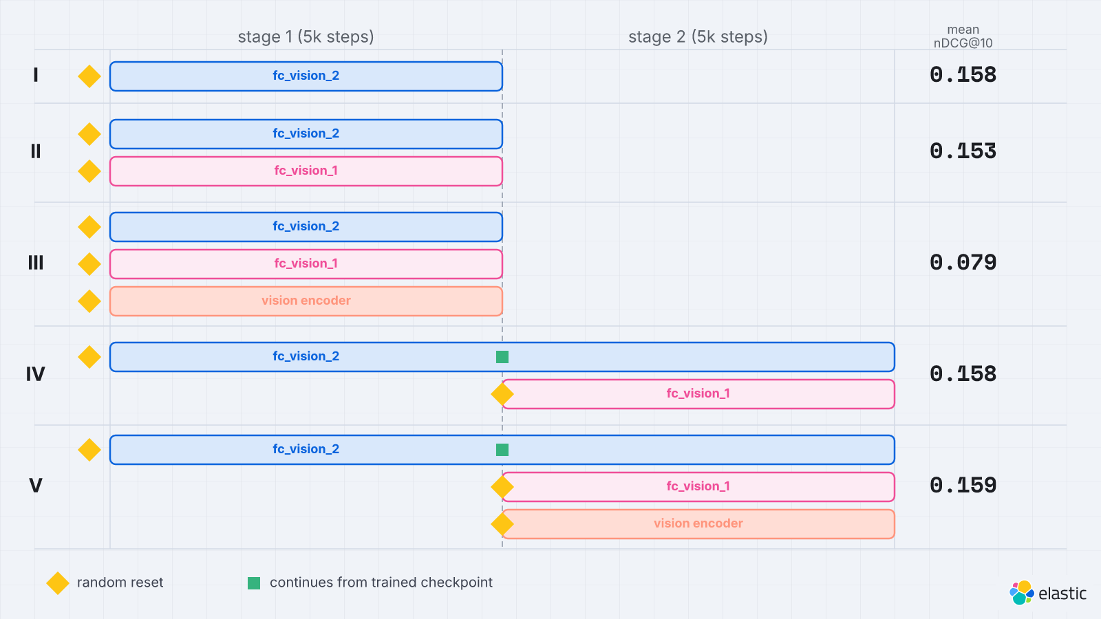
Overall, nearly every ablation study yielded basically identical results, except for case #3, which performed terribly. Before we explain why, let's look at the equivalent ablation diagram for audio.
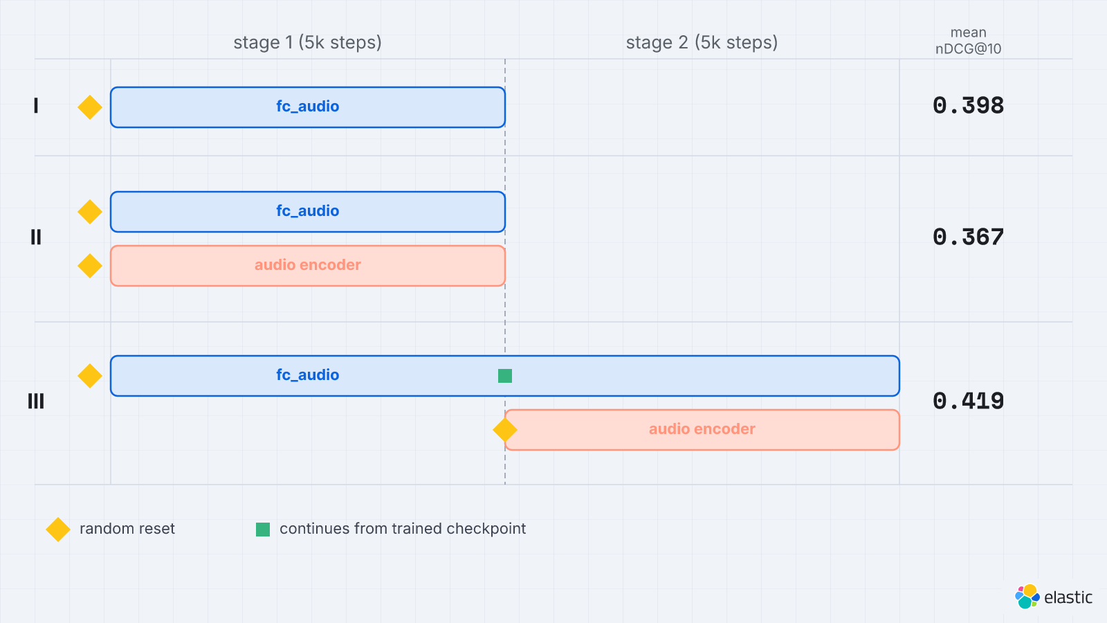
In this instance, ablation case #2 performs the worst. Do you see the commonality between the worst performer here and the worst performer among the vision ablations? Across both modalities, the same rule holds: If you unfreeze the encoder before the projector has been trained, you’ll see worse performance.
For both modalities, we ultimately chose ablation case #1 for the final architecture. Both had relatively high scores. In vision's case, the configurations that edged out case #1 did so by margins too small to justify their added training stages and extra per-task artifacts. A similar story unfolds for audio, with case #3 beating out case #1 by a small margin but requiring more per-task artifacts.
Ablation validates the GELATO approach: It's cheaper and nearly identical in quality to train a dedicated translator (rather than the speaker).
Summary: why frozen encoders make multimodal embeddings cheaper
Rather than expensively retraining multiple towers to achieve multimodal capabilities, GELATO allows us to minimize cost by freezing our already functioning towers and training only small projectors to translate embeddings. These embeddings get funneled into jina-embeddings-v5-text, ultimately allowing all the output vectors to exist in the same, interleaved geometry. We can now compare text, audio, images, and video at a fraction of the cost of the competition.
Both jina-embeddings-v5-omni-small and jina-embeddings-v5-omni-nano are open-weight for personal use and available now. You can download them from the Jina AI collection on Hugging Face and start generating multimodal embeddings today, or read the full technical report for the complete set of benchmarks and ablations.