What Are You Breathing: Analyzing Air Quality Data with Elasticsearch on Elastic Cloud (Part 1)
Want to learn more about the differences between the Amazon Elasticsearch Service and our official Elasticsearch Service? Visit our AWS Elasticsearch comparison page.
The Elastic Stack has proven to be more than up to the task of collecting, indexing, and providing insightful information from data. Integrated information management is not only possible, but as we’ll see over this series of posts, it can be a pleasant mission. We’ll walk the whole path from raw and meaningless data to conclusions any modern city dweller can use to improve their daily life.
The increasing population in main cities across the world poses many challenges. Among these, air pollution is probably one of those with more impact on their inhabitants’ health. In an effort to alert citizens and take emergency measures, some public institutions have deployed sensor fields that harvest information about the concentration of different pollutants across the city.
Since these measurements are a responsibility of public institutions, it is not unusual that they get published for anyone to make use of them. That is the case of samples taken at the third-largest european city (by population, with over three million inhabitants): Madrid.
Let’s see how easy it is to use Elasticsearch to make these, otherwise opaque chemical measurements talk about the customs of Madrid inhabitants.
From CSV Files to Elasticsearch Documents
First, we’ll need to take a look at the data source. Madrid’s City Hall maintains an Open Data Portal where it is possible to locate the hourly-air-quality-measurements data set (in Spanish).
There we can find an HTTP endpoint serving a CSV file which gets updated on an hourly basis and contains the measurements for the current day up to the last hour.
Each row of the file corresponds to a (Location, Chemical) key pair and contains the hour-by-hour measurements for a whole day. Each hour value is captured in a column.
| ... | STATION | CHEMICAL | ... | MONTH | DAY | 0 AM Measure | 0 AM Is valid? | ... | 11 PM Measure | 11 PM Is valid? |
| Number (Code) | Code (Code) | Number | Number | Number | 'V' or 'F' (True/False) | Number | 'V' or 'F' (True/False) |
Fields such as STATION and CHEMICAL are given as numeric values associated with geographical positions and compound formulation respectively. That association is provided via tables present at the data source site.
On the other hand, hourly measurements (i-th AM/PM Measurement) and flags indicating if they are valid (i-th AM/PM Is Valid?) are given as raw values. Units are provided by another table of the source specification while the validation flag can take `V` or `F` values representing the words “Verdadero” and “Falso” (“True” and “False” in Spanish).
Chemical sampling results are represented as measurements in space and time. Does that ring a bell? You got it right: time series of spatial events! That means rows are not events. On the contrary, up to 24 events are collected in each row — all of them sharing the same location and chemical compound.
If we encoded each event as JSON documents, they would look like the following example:
{
  "timestamp": 1532815200000,
  "location": {
    "lat": 40.4230897,
    "lon": -3.7160478
  },
  "measurement": {
    "value": 7,
    "chemical": "SO2",
    "unit": "μg/m^3"
  }
}
Optionally we could effortlessly enrich it with the World Health Organization (WHO) limits by just adding an additional field within the measurement sub-document. Breaking each CSV row into separate JSON documents makes them easier to understand, and even easier to ingest into Elasticsearch.
{
  "timestamp": 1532815200000,
  "location": {
    "lat": 40.4230897,
    "lon": -3.7160478
  },
  "measurement": {
    "value": 7,
    "chemical": "SO2",
    "unit": "μg/m^3",
    "who_limit": 20
  }
}
The set of all documents matching this structure can be described using another JSON document. This is a mapping in Elasticsearch and we will use it to describe how documents are stored in a given index.
{
  "air_measurements": {
    "properties": {
      "timestamp": {
        "type": "date"
      },
      "location": {
        "type": "geo_point"
      },
      "measurement": {
        "properties": {
          "value": {
            "type": "double"
          },
          "who_limit": {
            "type": "double"
          },
          "chemical": {
            "type": "keyword"
          },
          "unit": {
            "type": "keyword"
          }
        }
      }
    }
  }
}
Deploy a Cluster in Seconds on Elastic Cloud
At this point, you could either set up an Elasticsearch cluster locally or start a 14-day free trial of the Elasticsearch Service on Elastic Cloud. Learn how to spin up a new cluster with just a few clicks. For this demonstration, I’ll be using Elastic Cloud.
Once you’re logged into Elastic Cloud, you’ll need to deploy a new cluster. To size the cluster for this use case we should consider that a month’s worth of JSON measurement events file takes around 34 MB of disk space (before indexing), so we can use the smallest cluster offered (1 GB RAM/24 GB disk space). This small cluster should be enough to initially host our data. Elastic Cloud makes scaling easy, so if needed, we can always increase this size later, as well as change the number of availability zones or perform other changes in our cluster.
In less time than it takes to cook a microwave meal, we’ll have our Elasticsearch cluster ready to receive and index our collection of measure events.
Extract, Transform, and Load
Going from the original CSV file to a collection of JSON documents coding measurements isn’t a task anyone would like to manually perform (that sounds more like a sisyphean punishment). That’s a task to be automated.
For this, let’s start drafting an automation script to flatten the CSV table into JSON documents. Let’s use Scala to do that:
- As a language which allows centering on the data flow rather than on the program flow, it offers operations to easily transform collections of documents.
- It comes with lots of JSON manipulation libraries.
- Thanks to Ammonite, it is possible to write data manipulation scripts in the blink of an eye.
The following snippet of the extractor.sc script condenses the transformation logic:
  // Fetch the file from Madrid's city hall open data portal
  lazy val sourceLines = scala.io.Source.fromURL(uri).getLines().toList
  sourceLines.headOption foreach { head =>
    /* The CSV first line contains the columns labels, it is not difficult
       to compute a map from label to position thus making the rest of the code
       more readable. */
    lazy val label2pos = head.split(";").zipWithIndex.toMap
    // For each line, we'll produce several events, that's easilt via flatMap
    lazy val entries = sourceLines.tail flatMap { rawEntry =>
      val positionalEntry = rawEntry.split(";").toVector
      val entry = label2pos.mapValues(positionalEntry)
      /* The first 8 positions are used to extract the information common to the
       24 hourly measurements. */
      val stationId = entry("ESTACION").toInt
      val ChemicalEntry(chemical, unit, limit) = chemsTable(entry("MAGNITUD").toInt)
      // Measurement values are contained in the 24 last columns
      positionalEntry.drop(8).toList.grouped(2).zipWithIndex collect {
        case (List(value, "V"), hour) =>
          val timestamp = new DateTime(
            entry("ANO").toInt,
            entry("MES").toInt,
            entry("DIA").toInt,
            hour, 0, 0
          )
          // And there it go: The generated event as a case class!
          Entry(
            timestamp,
            location = locations(stationId),
            measurement = Measurement(value.toDouble, chemical, unit, limit)
          )
      }
    }
- Fetch the last published hourly report — containing the measurements taken up to an hour ago.
- For each row:
- Extract the fields common to all the events generated from the row — station id and measured chemical.
- Extract the measurements corresponding to the ones taken so far during the day (up to 24). Filter out those not labeled as valid measurements.
- For each of these, generate the measurement timestamp as the composition of the row date and the measurement column number. Combine the row common fields, the timestamp, and the registered value into a single event object (Entry).
The script continues serializing Entry objects as JSON documents and printing them as a succession of independent JSONs.
Extractor.sc can receive arguments to instruct it to fetch the data to transform from other sources, such as local files, or to add actions required by Elasticsearch’s Bulk API when uploading whole day files a time.
extractor
  --uri        String (default http://www.mambiente.munimadrid.es/opendata/horario.csv)
  --bulkIndex
  --bulkType
Upload Your Data to Elasticsearch
So we’ve just got a script which does the translation from CSV files to lists of documents. How can we index them? Easy, we have just to make a couple of calls to our cluster.
Index Creation
First things first: We need to create the index. We already came up with a JSON for our document mappings and we can nest it within our index definition: ./payloads/index_creation.json
{
    "settings" : {
        "number_of_shards" : 1
    },
    "mappings" : {
        "air_measurements" : {
            "properties" : {
                "timestamp": { "type": "date" },
                "location" : { "type" : "geo_point" },
                "measurement": {
                    "properties": {
                        "value": { "type": "double" },
                        "who_limit": { "type": "double" },
                        "chemical": { "type": "keyword" },
                        "unit": { "type": "keyword" }
                    }
                }
            }
        }
    }
}
Then ship it to our cluster’s index creation endpoint:
curl -u "$ESUSER:$ESPASS" -X PUT -H 'Content-type: application/json' \
     "$ESHOST/airquality" \
     -d "@./payloads/index_creation.json"
After which we’ll end up with the airquality index.
Bulk Upload
The fastest way to load all that data into Elasticsearch is with the Bulk API. The idea is to establish a connection, upload a package of documents, and finish the operation. If we did the upload one document at a time, we would have to establish a TCP connection, send the document, receive confirmation, and close the connection for every measurement in every row of the CSV! That’s too inefficient for me.
As the Bulk API documentation establishes, you are required to upload a NDJSON file with two lines per document:
- One with the action to perform at Elasticsearch
- A second with the document affected by that action. The action we’re interested in is index.
Thus extractor.sc comes with two additional options to control of the index action and its appearance right before each document:
- bulkIndex INDEX — If passed, it makes the extraction script to precede each document by an index into INDEX action.
- bulkType TYPE — If passed after bulkIndex, completes the index action with the type the document should match.
    /* The collection of events is then serialized and printed in the standard ouput.
       That way, we can use them as a ndjson file.
     */
    val asJsonStrings = entries flatMap { (entry: Entry) =>
      Some(bulkIndex).filter(_.nonEmpty).toList.map { index =>
        val entryId = {
          import entry._
          val id = s"${timestamp}_${location}_${measurement.chemical}"
          java.util.Base64.getEncoder.encodeToString(id.getBytes)
        }
        /* Optionally, we can also serialize bulk actions to improve data transfer
           performance. */
        BulkIndexAction(
          BulkIndexActionInfo(
            _index = index,
            _id = entryId,
            _type = Some(bulkType).filter(_.nonEmpty)
          )
        ).asJson.noSpaces
      } :+ entry.asJson.noSpaces
    }
    asJsonStrings.foreach(println)
This way we can generate our giant NDJSON file with all the entries for the day:
time ./extractor.sc --bulkIndex airquality --bulkType air_measurements > today_bulk.ndjson
Taking 1.46 seconds, it has generated the file we can send to the Bulk API as follows:
time curl -u $ESUSER:$ESPASS -X POST -H 'Content-type: application/x-ndjson' \
     $ESHOST/_bulk \
     --data-binary "@today_bulk.ndjson" | jq '.'
The upload request took 0.98 seconds to complete.
The total time for this method took 2.44 seconds (1.46 seconds from data fetching and transformation plus 0.98 seconds from the bulk upload request), which is 182 times faster than if we uploaded one document at a time. That’s right, 2.44 seconds vs. 7 minutes and 26 seconds!
An important takeaway here is: Use bulk uploads for processes indexing larger quantities of documents!
From Data to Insight
Congratulations! We’ve reached the point where we have our city’s air measurements indexed in Elasticsearch. That means, for example, we can easily search and fetch the data much more easily than having to download, extract, and manually search the information we are looking for.
Take this case as an example — If after enjoying the contemplation of Las Meninas, we had to choose whether to:
- Spend some time enjoying Madrid’s sunny outdoors
- Keep having a great time at El Prado museum
We could ask Elasticsearch which option would be better for our health by requesting it to tell us what was the latest NO2 measurement taken at the closest weather-station within 1 km: ./es/payloads/search_geo_query.json
{
  "size": "1",
  "sort": [
    {
      "timestamp": {
        "order": "desc"
      }
    },
    {
      "_geo_distance": {
        "location": {
          "lat": 40.4142923,
          "lon": -3.6912903
        },
        "order": "asc",
        "unit": "km",
        "distance_type": "plane"
      }
    }
  ],
  "query": {
    "bool": {
      "must": {
        "match": {
          "measurement.chemical": "NO2"
        }
      },
      "filter": {
        "geo_distance": {
          "distance": "1km",
          "location": {
            "lat": 40.4142923,
            "lon": -3.6912903
          }
        }
      }
    }
  }
}
curl -H "Content-type: application/json" -X GET -u $ESUSER:$ESPASS $ESHOST/airquality/_search -d "@./es/payloads/search_geo_query.json"
And receive the following answer:
{
  "took": 4,
  "timed_out": false,
  "_shards": {
    "total": 1,
    "successful": 1,
    "skipped": 0,
    "failed": 0
  },
  "hits": {
    "total": 4248,
    "max_score": null,
    "hits": [
      {
        "_index": "airquality",
        "_type": "air_measurements",
        "_id": "okzC5mQBiAHT98-ka_Yh",
        "_score": null,
        "_source": {
          "timestamp": 1532872800000,
          "location": {
            "lat": 40.4148374,
            "lon": -3.6867532
          },
          "measurement": {
            "value": 5,
            "chemical": "NO2",
            "unit": "μg/m^3",
            "who_limit": 200
          }
        },
        "sort": [
          1532872800000,
          0.3888672868035024
        ]
      }
    ]
  }
}
Telling us that the weather station at El Retiro reports 5 μg/m^3 of NO2. Not a bad result taking into account that the WHO limit is 200 μg/m^3, so let’s go have some tapas!

To be honest, I’ve never found anyone pulling a laptop out and start writing cURL commands within the museum. However, these requests are so easy to code in almost any programming language that it’s possible to provide frontend applications in a few days. That is, we already have a full-fledged analytics back end with our information index.
Visualizing the Invisible with Kibana
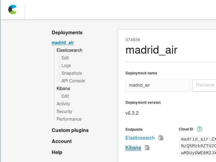
What if we didn’t need to write the application at all? What if, with the current cluster, we could start exploring the data by clicking our way into insightful information? Thanks to Kibana, that’s definitely possible. We can go to our cluster management at cloud.elastic.co, and click on the link giving us access to our Kibana deployment:
With Kibana, we can create comprehensive visualizations and dashboards fed with the documents indexed in Elasticsearch.
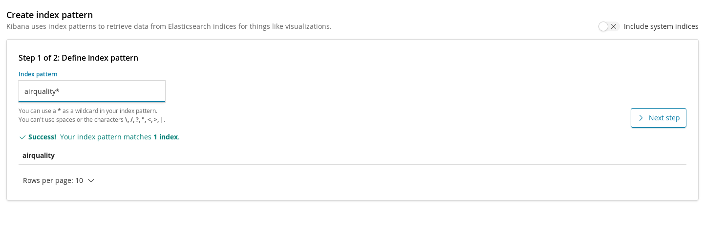
Index patterns are the way we have to register indices into Kibana so they can be used by visualizations to pull data. Therefore, the first step before creating charts for our airquality index is to register it.
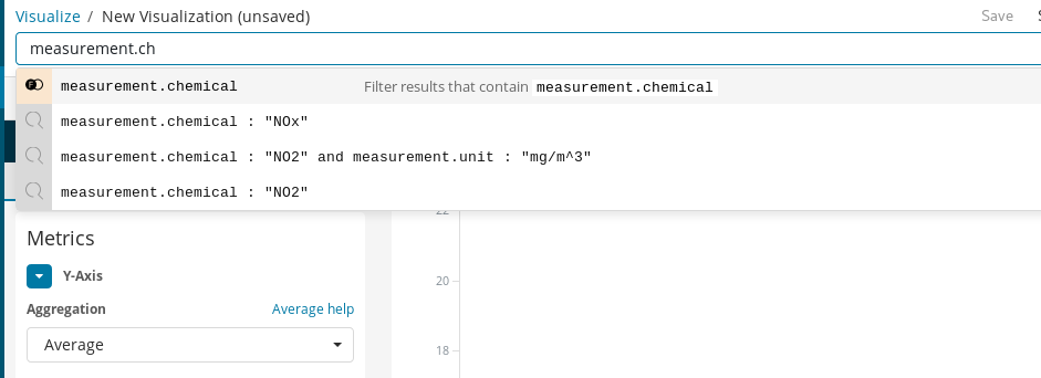
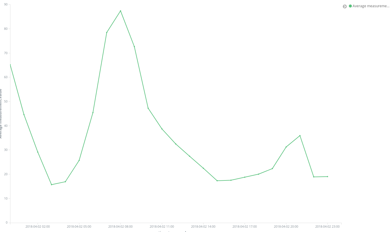
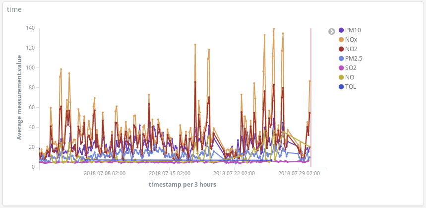
Once created, we can add our first visualization. Let’s start with something simple: Plotting the evolution over time of the average concentration levels across the city for a chemical. Let’s do it for NO2:
First, we need to create a Line Chart where Y-Axis is an Average aggregation for the field measurement.value over hourly buckets represented on the X-Axis. To select the target chemical we can use Kibana’s query bar which makes it easy to filter NO2 measurements and, by enabling autocomplete, we can get suggestions guiding us through the query definition process.
Finally, with Time Range we choose the timespan of the visualized data.
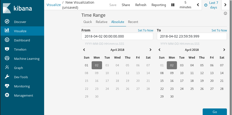
Few clicks, immediate results:
One of the more insightful charts we can use for this dataset are Coordinate Maps. As each measurement comes with the coordinates of the station which captured it, we can represent pollution hotspots. That is, shifting from averaging spatial entries in time buckets to averaging time entries in spatial locations. So the buckets are now Geohash aggregations over location, the field containing the point of measurement.
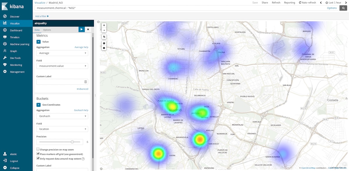
If we select the last hour time range, we can get an idea of what are the cleaner areas to visit at this time. Yearly time ranges tell us what are the cleaner areas on average and can help us, for example, to take a decision on where to buy a house to live a healthier life.
Scripted Fields
Since our documents piggy back the WHO recommended levels for some chemicals, it is possible to visualize how unhealthy is the air. One way to do this is by using gauge visualization over the proportion of a measured level and the WHO limit. But that division wasn’t performed when we loaded the data. That’s not a problem as it is still possible to generate new fields from the indexed ones using the Painless scripting language, which is easy to understand and write by anyone who has ever used Java (since Kibana 6.4, it is also possible to get a preview of the results yielded by the Painless script).
Then use them in our visualizations as if they were regular indexed fields:
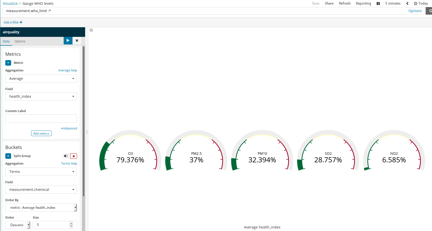
It is worth noting how simple rules yield rich visualizations in Kibana. In the example above we:
- Filtered documents — selecting only those for which there are WHO limits.
- Used Split Groups and Term Aggregation over
measurement.chemical.
Thus generating a gauge graph for each chemical for which there known WHO limits.
Learning About Pollution in Madrid
Kibana visualizations can be leveraged to build dashboards that aggregate visualizations, which is key to interpret and understand the state of a system in real time. In this case, the system is the atmosphere composition and its interactions with human activities.
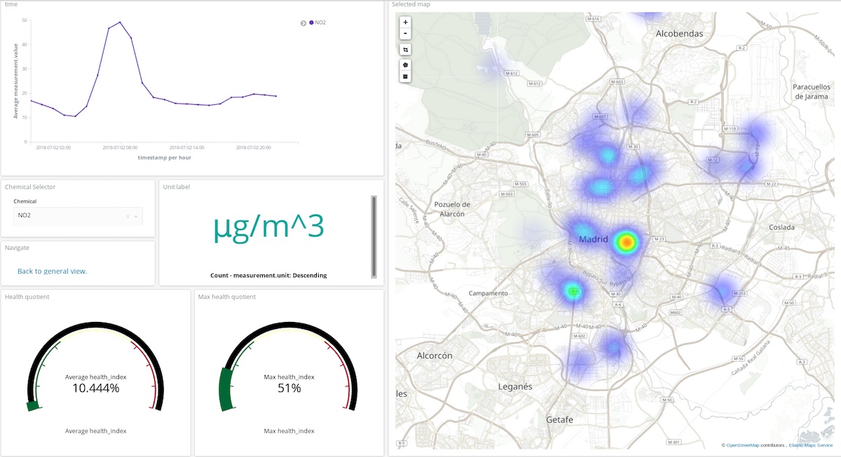
In the dashboard above, a user can pick any chemical, a time period and get a pretty good idea of where and in what quantity that compound is polluting the atmosphere. Take a look yourself! (user: test, password: madrid_air).
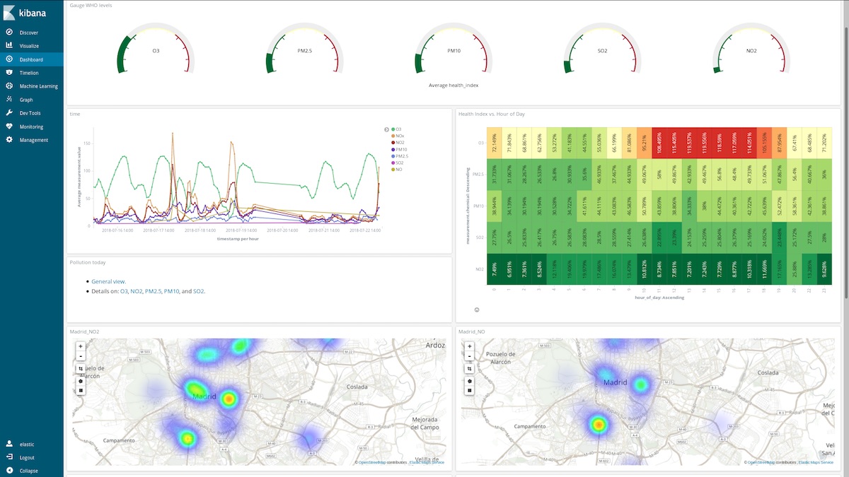
It is also possible to get a general idea (same user and password) of Madrid’s air quality.
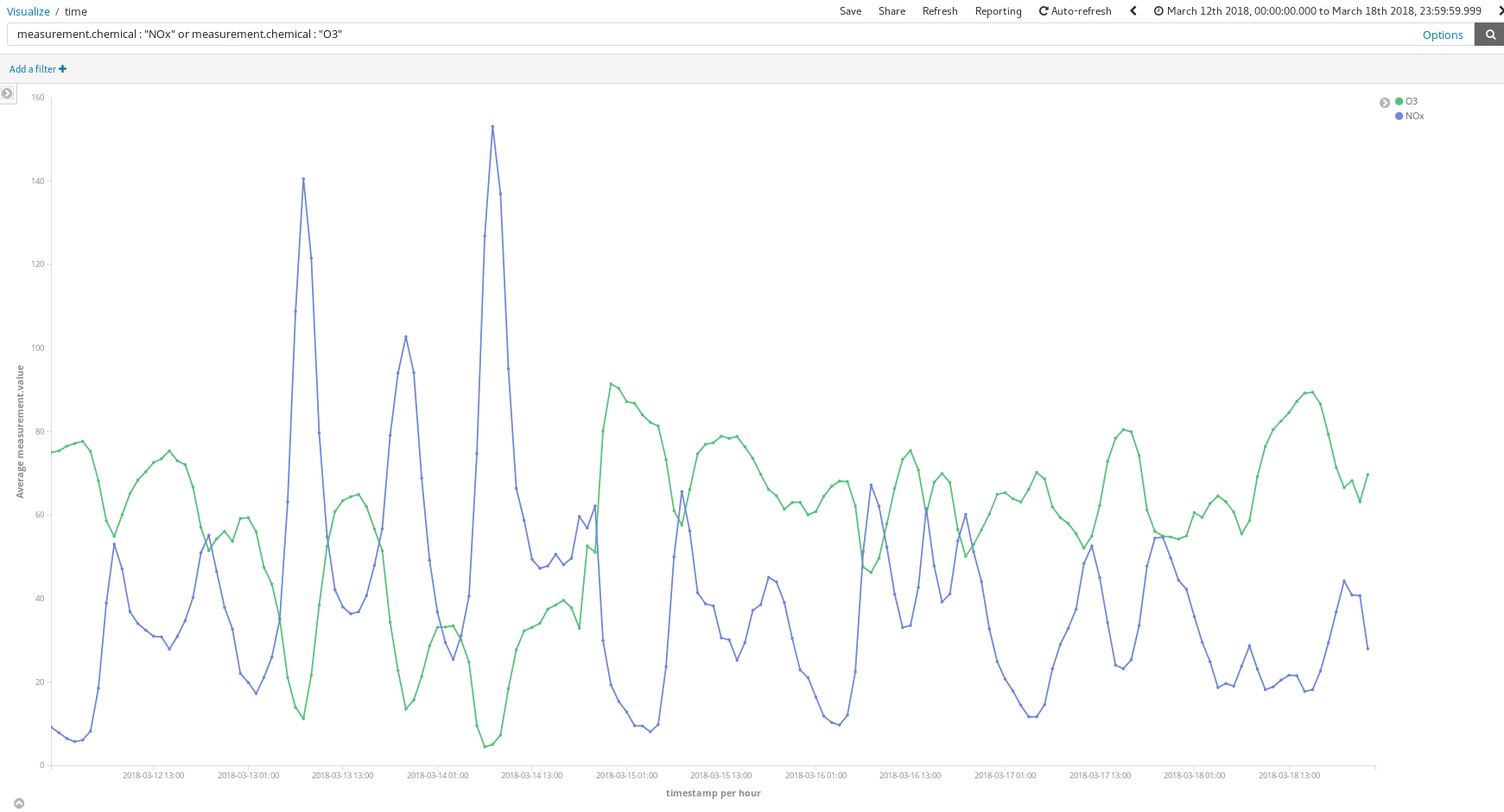
How do these dashboards help? Let’s take a look at any random week in March (From March 12 to March 18):
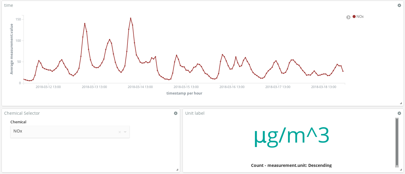
Do these NOx (a compound produced by combustion in diesel engines) peaks tell us something about Madrid citizens habits? Indeed, they do. They occur twice per day…
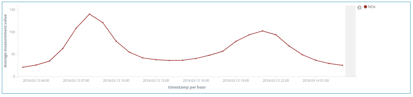
One around 8 am CEST and the second around 9 pm CEST. What we see here is the increasing use of diesel cars to move across the city when workers head to their workplaces. Almost no one uses them during working hours, and there is a surge of smoke when they finish their work at the office and go back home.
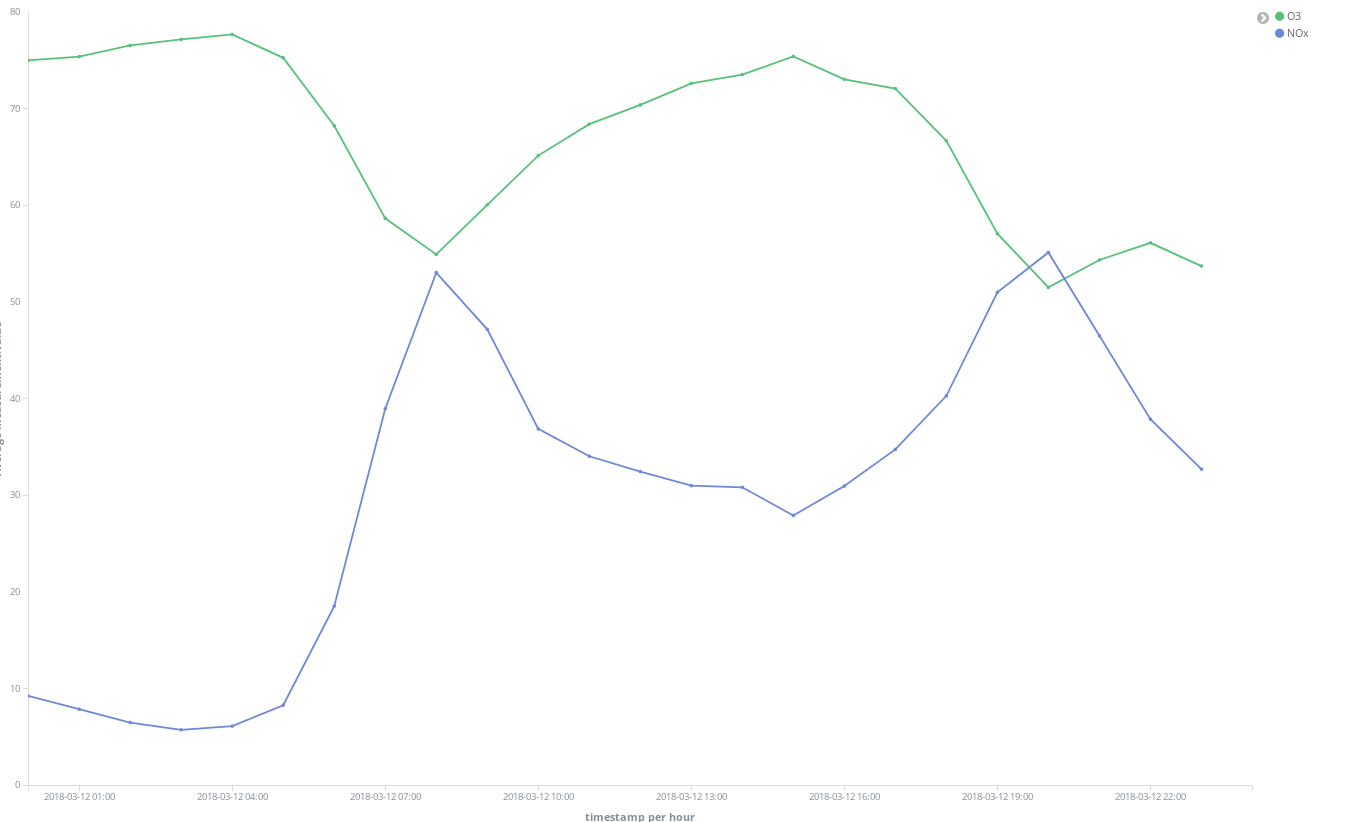
It is also interesting to see how O3 concentration increases as NOx reduces. O3 is a by-product of the reactions between NOx and organic compounds in the presence of sunlight so a correlation of NOx and O3 is expected.
We can also find that the general situation improves on weekends:
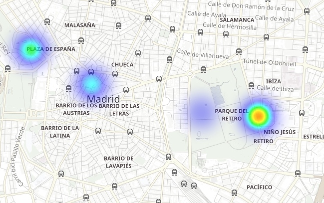
See how El Retiro park (a huge green area within the heart of the city) is surrounded by NO2 emissions hotspots while being a lower emissions area itself due to thick vegetation and lack of traffic:
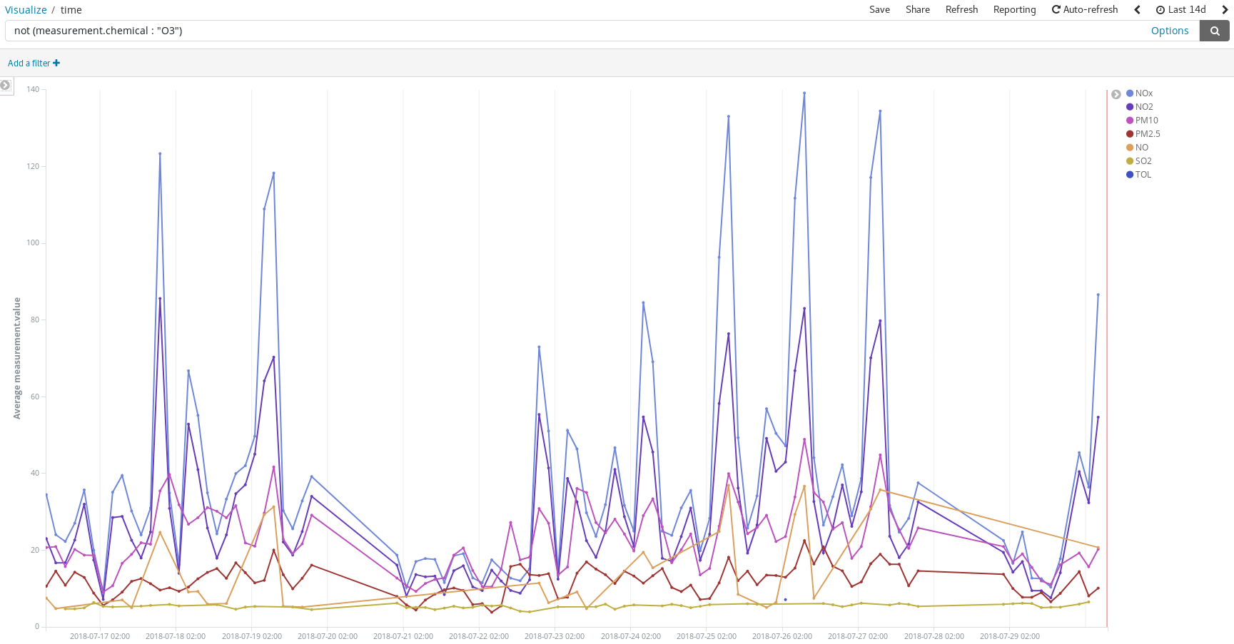
Detect pollution peaks on the days people usually take their cars to their summer vacation destinations:
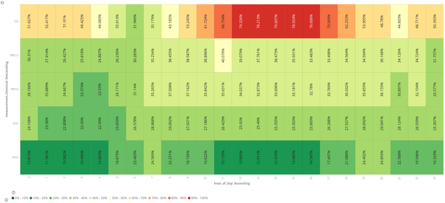
Or add an additional scripted field (hour_of_day) to bucket out entries in hours to present the average measurements, by chemical, in a heatmap. It seems 6 am is the best time to schedule a running session:
At the end of the day we got convinced that there is more in the air than just Nitrogen, Oxygen, Carbon Dioxide, Argon, and water. So no! It is not just air what we are breathing when we walk down Gran Via in Madrid. And probably not when you are exploring Manhattan, feeling like checking by yourself? You now know the path, an open data source is what it takes to start.
Conclusion
If we were data engineers asked to set up tools for our company’s data scientists to analyze pollution levels in Madrid, we would have finished our job when we registered the airquality index pattern in Kibana, wrapped the access link in an email, and let them play with it. The Elastic Stack offers a full analytics stack from where it is possible to get answers in minutes and in a very intuitive way where the only code to write is that one of the scripted fields (when needed).
Thanks to Elastic Cloud, our job as data engineers has been simplified to just a few clicks and writing the Extract Transform Load (ETL) service. But, would we actually need to write an ETL to fetch and get our data into Elasticsearch? Next post will show that the Elastic Stack can also take care of that.