Managing data automation through hot, warm, cold, and frozen tiers — No coding needed!

 Share on Twitter
Share on Twitter

 Share on LinkedIn
Share on LinkedIn

 Share on Facebook
Share on Facebook

 Share by Email
Share by Email

 Print this page
Print
If you are looking to do exactly what the title of this article suggests, look no further. This post intends to be a guide on how one can use the Kibana Dashboard’s “Stack Management” feature-set to automate the movement of your data through hot, warm, cold, and frozen tiers, without the need to do any coding or execute command-line actions.
Before we begin: Core concepts
Let’s take a step back to understand some core concepts of how data sits and moves within your Elasticsearch cluster before we go into how you can automate its movement. This is so we will be familiar with certain terms and patterns later on when we go into the hands-on step-by-step process in practice.
If your organization stores data, you will definitely need to consider a technical concept called “High Availability” or “Redundancy” — in simple terms, it means keeping multiple copies of the original data to prevent data loss if a single part of your distributed system fails. Gone are the days where one’s data sits in just a single datacenter, where it is prone to data loss or unavailability due to possible failures.
In this day and age, it is an industry practice to ensure that your data is highly available, meaning you should be able to access it on a 24/7 basis and it should be resilient to failures. This is where the concept of data partitioning comes in, which is to split your table(s) (also known as an “index” or “indices”) into multiple parts so they can be distributed across different datacenters.
Why do we need to understand this? For data to move, they have to be partitioned.
In online Cloud terms, these data centers across different areas are known as “Availability Zones” (AZs). The underlying systems that hold these blocks of data being synchronized in real-time are then called “nodes,” which are a part of a “cluster.” A cluster is a collection of nodes that intelligently operate together. When the systems detect that a replicated part of the original data is missing, it will “auto-heal” by quickly replicating that data and copying it onto other nodes to make sure that at any point of time, there is more than one copy of the original data stored in the cluster.
In addition, there is also the concept of “Rollovers” — essentially, if a single data table (i.e., an index in Elasticsearch) gets too large, it can be partitioned into multiple smaller data tables that are internally further partitioned again (called “Shards” in Elasticsearch terms). In essence, “Rollovers” are a way to move data into smaller tables, which can then be moved easily within Elasticsearch — or more specifically, the “shards” of these tables are moved. We’ll go into more detail on this concept in the next section.
[Related article: How many shards should I have in my Elasticsearch cluster?]
Using an analogy: Excel spreadsheet workbook
Imagine your data to be like a giant Excel spreadsheet workbook. When we talk about “high availability,” imagine the data inside this Excel spreadsheet workbook being replicated into two copies. These two copies of data are then broken down into many smaller workbooks that are then somehow able to sync in real-time across different employees’ laptops.
This concept in an Elasticsearch database is called a “cluster,” where copies of your data are able to sync in real-time across different “nodes.”
Coming back to the Excel spreadsheet workbook analogy: if one employee’s laptop somehow breaks, there is still a copy of a part of the original data on another employee’s laptop, and that data is still “available.” This employee who now holds the single copy of original data then quickly copies it and distributes it to another employee’s laptop, so that at any point of time, there is more than one copy of that part of the original data. This is what it means to be “highly available.”
In Elasticsearch Database terms, this is called “sharding,” which is Elastic’s way of partitioning the data so that these partitioned data “shards” can be distributed across different data “nodes” sitting in different datacenter “zones.”
For an excel spreadsheet workbook, remember how you are able to have many “tab sheets”? Continuing from the analogy above, if one sheet gets too large — say, above 10,000 in rows total — then the employees will rollover this data by creating a new sheet tab and insert data into that new sheet tab instead! This ensures easier searching of data. Rather than having to look through 1 million rows of data in a single table, employees can have multiple spreadsheet tabs of only 10,000 rows each to search through, which makes searching more efficient.
This concept was an analogy of what we have in Elasticsearch Database, better known as Elastic “Data Streams,” which is essentially a collection of rollover tables (“indices”).
Since we now understand the concept of “high availability,” “shards,” and “rollovers,” and how these are useful in partitioning data, let’s move on to how to actually set this up in Elasticsearch using the Kibana User Interface (UI) Dashboard.
Complex, made simple: Step-by-step guide
Your data can be managed by utilizing a combination of Elastic “Data Streams,” “Index Templates,” and “Index Lifecycle Policies,” all within Kibana without the need to do any coding. Without further ado, let’s step through how this can be done:
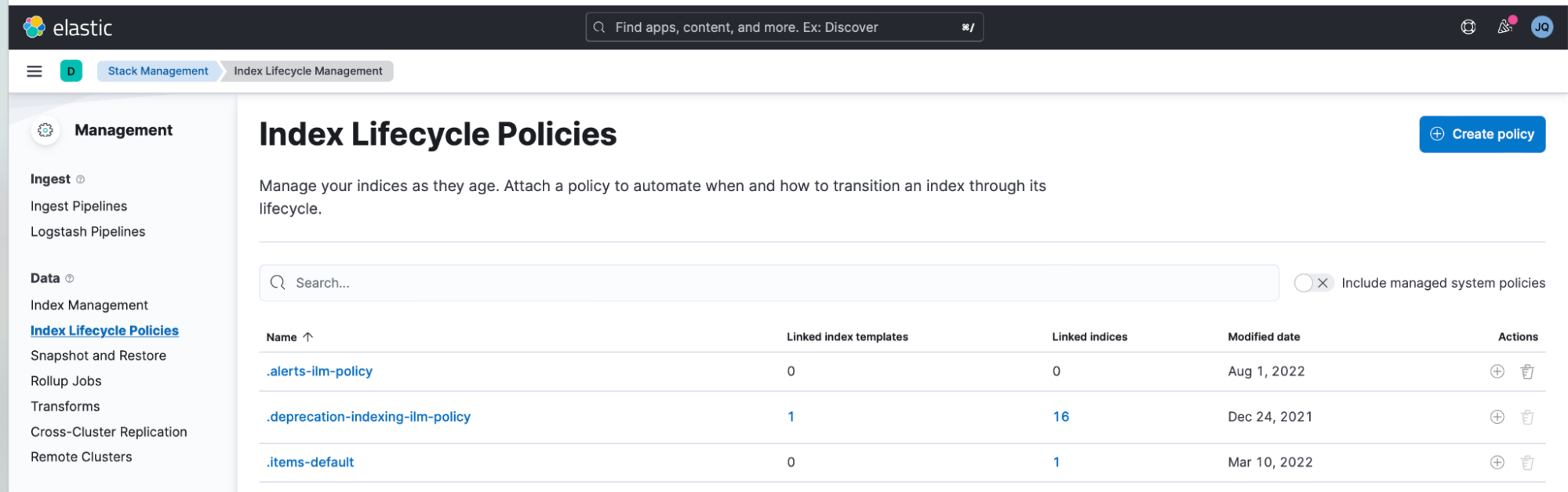
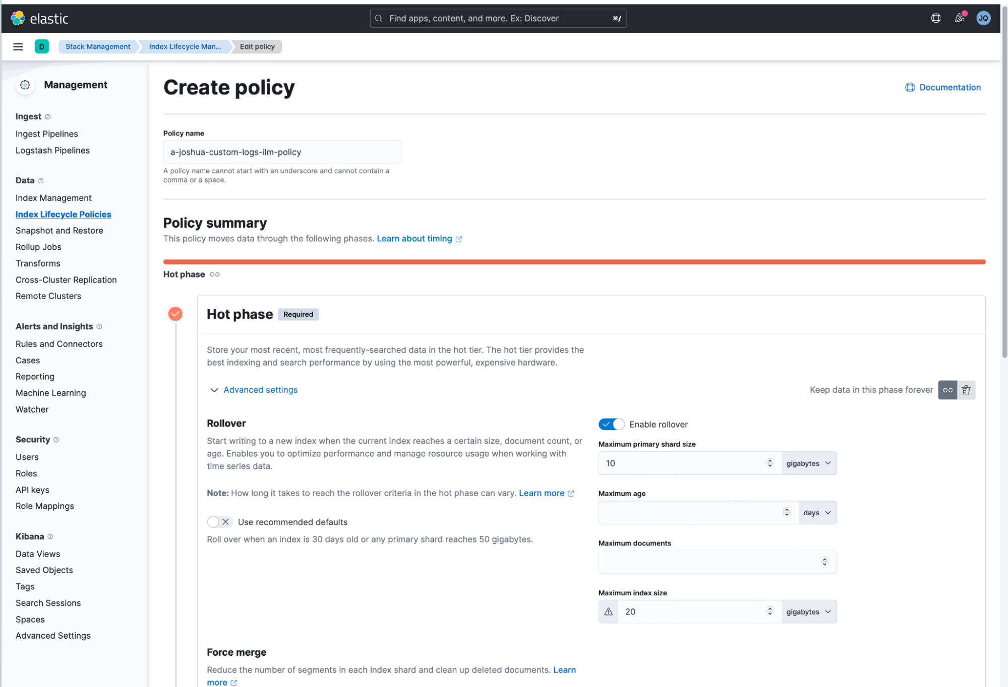
1. The first step is to log in to Kibana, open the left menu, and select “Stack Management.” Next, create an Index Lifecycle Management Policy by navigating to Index Lifecycle Policies > Create Policy. This is the mechanism that helps ensure that your data is in bite-sized pieces for more efficient searching.
- In the example screenshots, I named mine “a-joshua-custom-logs-ilm-policy.”
- Also set the maximum shard size to 10GB and maximum index size to 20GB.
- This will fully ensure every index created will be capped at a maximum of 20GB, and the index’s shards will be capped at a maximum size of 10GB (assuming that the original copy index data is replicated only once, which occurs by default.) As explained previously, this configuration is important because a collection of many smaller indices is more easily searchable than a single huge index.
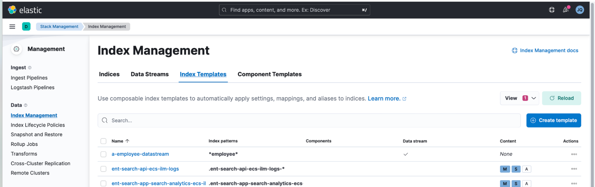
2. Create an Elastic "Index Template" here using Kibana > Index Management > Index Templates > Create template.
- Tick the "Create Data Stream" switch in the screenshot. Remember, an Elastic “Data Stream” is a collection of “indices.”
- In this example, I named this Index Template as “a-joshuaquek-datastream-creation-template.”
- Click all the way and press Done to create the Index Template.
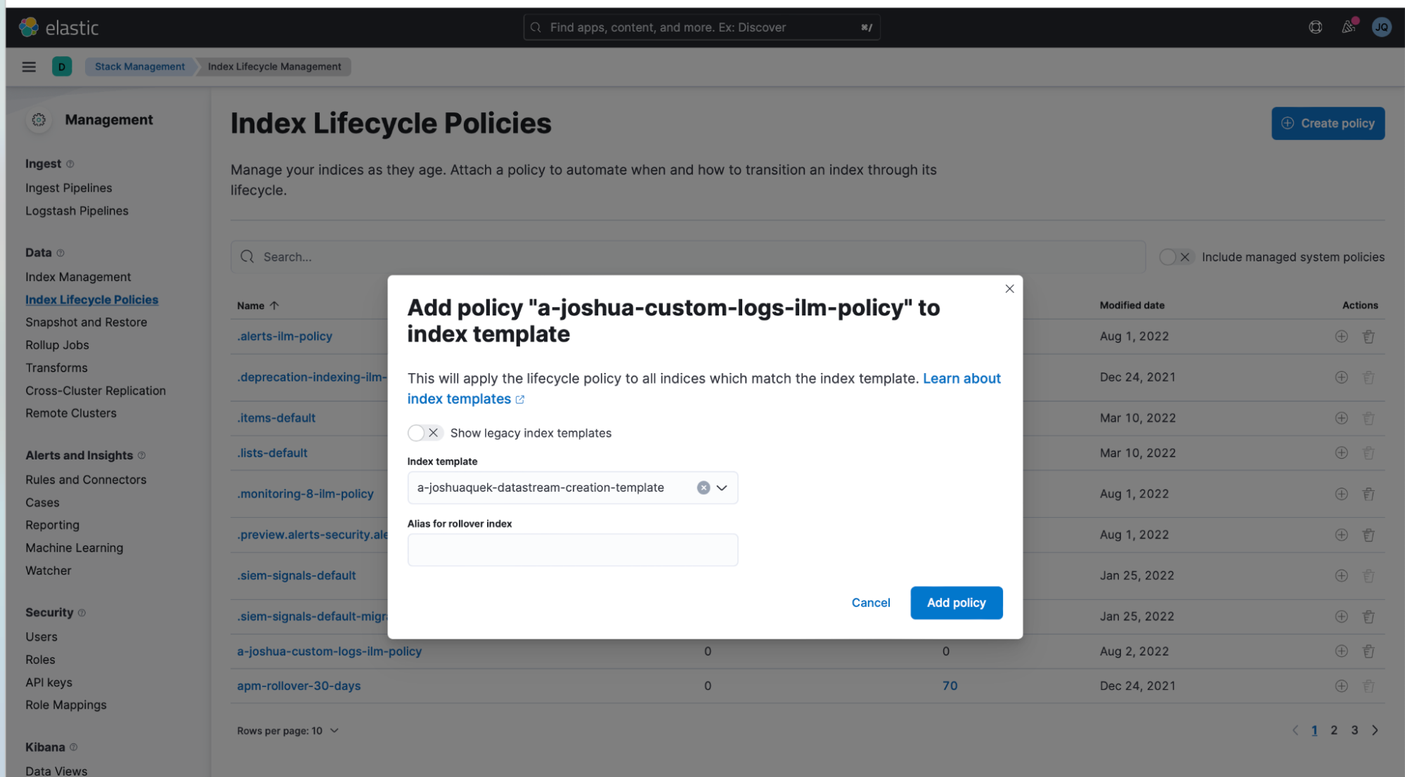
3. Now go back to your "Stack Management > Index Lifecycle Policies."
- In my example, I attached it to the a-joshua-custom-logs-ilm-policy that I created earlier in Step 1.
- Press the (+) button beside the lifecycle policy and attach it to the Index Template.
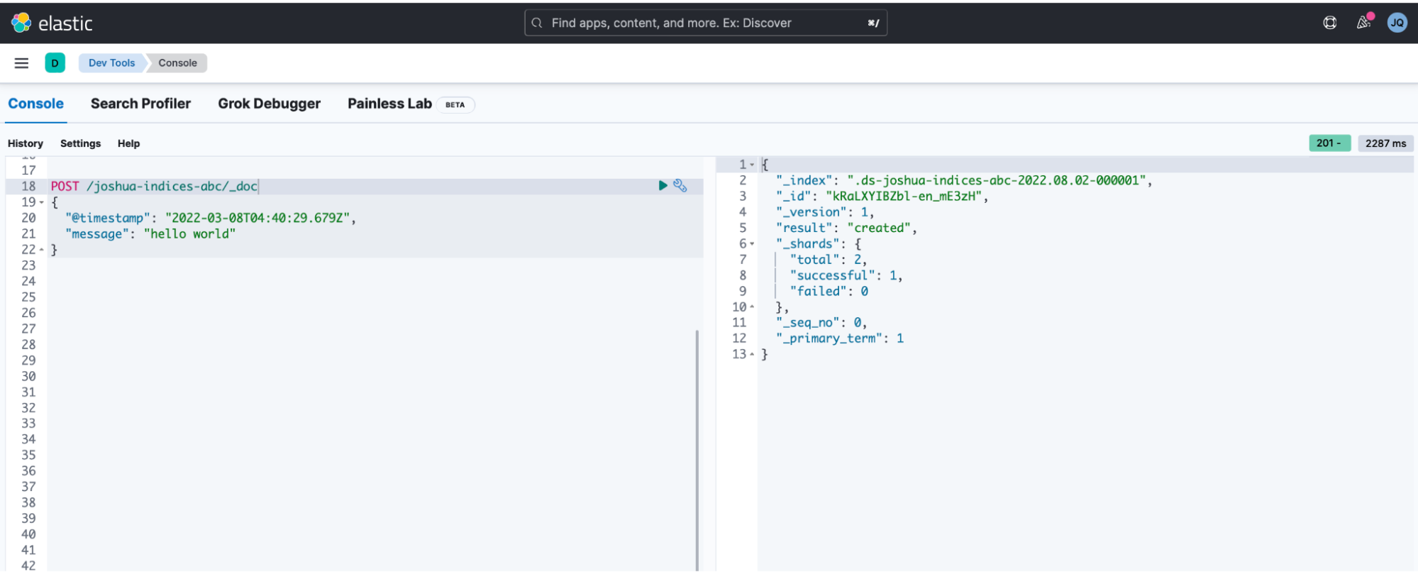
4. Test that this works by simulating ingestion of some example data.
- Go to the "Management > Dev Tools" and try ingesting one document — this creates the actual data stream.
POST /joshua-indices-abc/_doc
{
  "@timestamp": "2022-03-08T04:40:29.679Z",
  "message": "hello world"
}- In my example, I am ingesting a document into a new datastream that I am naming as joshua-indices-abc.
- You can see "result": "created" that shows that you have successfully created your data stream.
5. Now go back to the "Stack Management > Index Management > Datastream," and you can see that a data stream has been created!

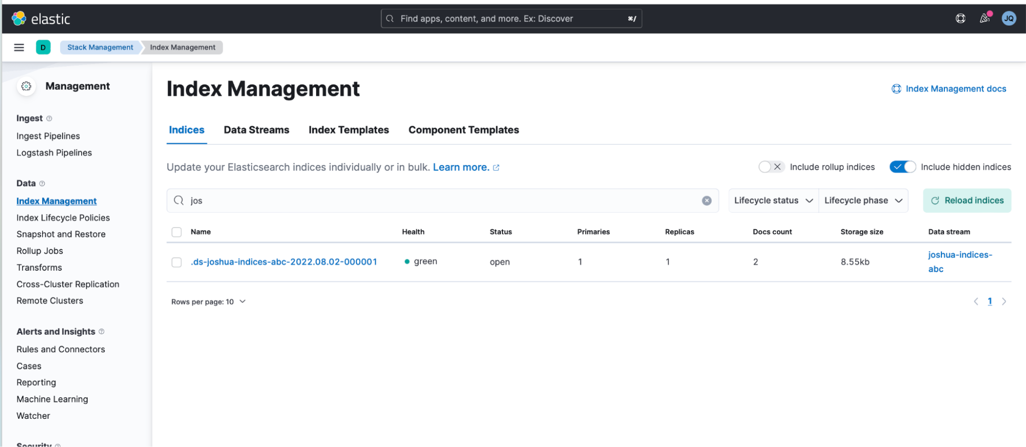
6. Go to "Stack Management > Index Management > Indices.
- You will notice that .ds-joshua-indices-abc-2022.08.02-000001 was created.
- Tick the "Include hidden indices," option and then search for index that gets generated by the data stream (collection of indices).
7. Over time, your data stream will grow. Since a data steam is essentially a collection of indices, it will internally create new backing indices based on the index lifecycle policy that you set earlier:
.ds-joshua-indices-abc-2022.08.02-000001
.ds-joshua-indices-abc-2022.08.02-000002
.ds-joshua-indices-abc-2022.08.02-000003
.ds-joshua-indices-abc-2022.08.02-000004
…
…
Notice that these backing indices get created based on the date and an incremented serial number. This serial number starts at 000001 and will increment every time a new backing index is created. You can read more about these here (visual illustrations included too).
8. Each index in this collection of indices (which is called a "data stream") now has a maximum shard size of 10GB and maximum index size of 20GB! Never again will you have to deal with overly large indices or shard sizes that belong to this collection of indices.
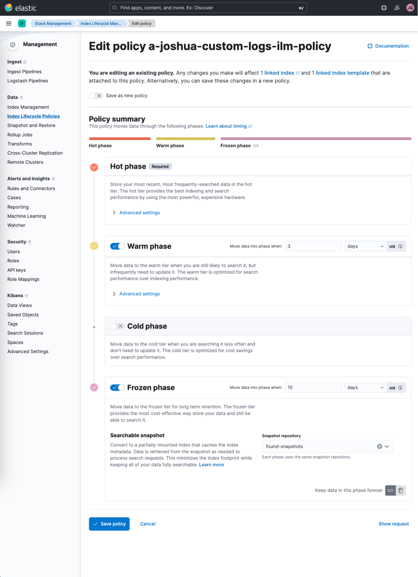
9. Once your setup is finished, if you wish to allow your indices to move to warm, cold, or even the frozen phase, head back over to "Stack Management > Index Lifecycle Management" and click on the Index Lifecycle policy you created in Step 1. Over there, you can optionally enable the different data tiers (warm, cold, frozen).
In summary
Overall, we have seen how one can harness Kibana as a powerful tool for managing your data — in this case, to control your index sizes within your Elasticsearch cluster using a combination of both Elastic “Data Streams,” “Index Templates,” and “Index Lifecycle Policies.” If you have enjoyed this short article and have not used Kibana nor Elasticsearch before, feel free to give it a test drive.
Share
- Share on Twitter
Share on Twitter
- Share on LinkedIn
Share on LinkedIn
- Share on Facebook
Share on Facebook
- Share by Email
Share by Email
- Print this page
Print