Elasticsearch has native integrations with the industry-leading Gen AI tools and providers. Check out our webinars on going Beyond RAG Basics, or building prod-ready apps with the Elastic vector database.
To build the best search solutions for your use case, start a free cloud trial or try Elastic on your local machine now.
With 8.2, the Elastic Stack gives users the random_sampler aggregation. It adds the capability to randomly sample documents in a statistically robust manner. Randomly sampling documents in aggregations allows you to balance speed and accuracy at query time. You can aggregate billions of documents with high accuracy at a fraction of the latency. This allows you to achieve faster results with fewer resources and comparable accuracy — all with a simple aggregation.
Let's run through some basic details, best practices, and how it works, so you can try it out in the Elasticsearch Service today.
Delivering speed and accuracy
Random sampling in Elasticsearch has never been easier or faster. If your query has many aggregations, you can quickly obtain results by using the random_sampler aggregation.
All the above aggregations nested under random_sampler will return sampled results. Each agg is roughly seeing only 0.1% of the documents (or 1 in every 1000th document). Where computational cost correlates with the number of documents, the aggregation speed increases. You may have also noticed the “seed” parameter. You can provide a seedto get consistent results on the same shards. Without a seed, a new random subset of documents is considered and you may get slightly different aggregated results.
How much faster is the random_sampler? The speed improves according to the provided probability as fewer documents are aggregated. The improvements relative to probability will eventually flatten out. Each aggregation has its own computational overhead regardless of the number of documents. An example of this overhead cost is comparing multi-bucket to single metric aggregations. Multi-bucket aggregations have a higher overhead due to their bucket handling logic. While speed is improved for multi-bucket aggregations, the rate of that speed increase will flatten out sooner than single metric.

Figure 1. The speedup expected for aggregations of different constant overhead.
Here are some results on expected speed and error rate over an APM data set of 64 million documents.
The calculations are from: 300 query and aggregation combinations, 5 seeds, and 9 sampling probabilities. In total, 13,500 separate experiments generated the following graphs for median speedup and median relative error as a function of the downsample factor which is 1 / sample probability.

Figure 2. Median speedup as a function of the downsample factor (or 1 / probability provided for the sampler).

Figure 3. Median relative error as a function of the downsample factor (or 1 / probability provided for the sampler).
With a probability of 0.001, for half of the scenarios tested, there was an 80x speed improvement or better with a 4% relative error or less. These tests involved a little over 64 million documents but spread across many shards. More compact shards and larger data can expect better results.
But, you may ask, do the visualizations look the same?
Below are two visualizations showing document counts for every 5 minutes over 100+ million documents. The total set loads in seconds and is sampled in milliseconds. This is with almost no discernible visual difference.

Figure 4. Sampled vs unsampled document count visualizations.
Here is another example. This time the average transaction by hour is calculated and visualized. While visually these are not exactly the same, the overall trends are still evident. For a quick overview of the data to catch trends, sampling works marvelously.

Figure 5. Sampled vs. unsampled average transaction time by hour visualization.
Best practices for using sampling aggregation
Sampling shines when you have a large data set. In these cases you might ask, should I sample before the data is indexed in Elasticsearch? Sampling at query time and before ingestion are complimentary. Each has its distinct advantages.
When sampling at ingest time, it can save disk and indexing costs. However, if your data has multiple facets, you have to stratify sampling over facets when sampling before ingestion, unless you know exactly how it will be queried. This suffers from the curse of dimensionality and you could end up with underrepresented sets of facets. Furthermore, you have to cater for the worst case when sampling before ingestion. For example, if you want to compute percentiles for two queries, one which matches 50% of the documents and one which matches 1% of documents in an index, you can get away with 7X more downsampling for the first query and achieve the same accuracy.
Here is a summary of what to expect from sampling with the random_sampler at query time.

Figure 6. Relative error for different aggregations.
Sampling accuracy varies across aggregations (see Figure 5 for some examples). Here is a list of some aggregations in order of descending accuracy: percentiles, counts, means, sums, variance, minimum, and maximum. Metric aggregation accuracy will also be affected by the underlying data variation: the lower the variation in the values, the fewer samples you need to get accurate aggregate values. The minimum and maximum will not be reliable with outliers, since there is always a reasonable chance that the sampled set misses the one very large (or small) value in the data set. If you are using terms aggregations (or some partitioning such as date histogram), aggregate values for terms (or buckets) with few values will be less accurate or missed altogether.
Aggregations also have fixed overheads (see Figure 1 for an example). This means as the sample size decreases, the performance improvement will eventually level out. Aggregations which have many buckets have higher overheads and so the speedup you will gain from sampling is smaller. For example, a terms aggregation for a high cardinality field will show less performance benefit.
If in doubt, some simple experiments will often suffice to determine good settings for your data set. For example, suppose you want to speed up a dashboard; try reducing the sample probability while the visualizations look similar enough. Chances are your data characteristics will be stable and so this setting will remain reliable.
Uncovering how sampling works
Sampling considers the entire document set within a shard. Once it creates the sampled document set, sampling applies any provided user filter. The documents that match the filter and are within the sampled set are then aggregated (see Figure 7).

Figure 7. Typical request and data flow for the random_sampler aggregation.
The key to the sampling is generating this random subset of the shard efficiently and without statistical biases. Taking geometrically distributed random steps through the document set is equivalent to uniform random sampling, meaning each document in the set has an equally likely chance of being selected into the sample set. The advantage of this approach is that the sampling cost scales with p (where p is the probability configured in the aggregation). This means no matter how small p is, the relative latency of performing the sampling adds will remain fixed.
Ensuring performance reliability and accuracy
To achieve the highest performance, accuracy, and robustness, we evaluated a range of realistic scenarios.
In the case of random_sampler, the evaluation process is complicated by two factors:
- It cuts right across the aggregation framework and so it needs to be evaluated with many different combinations of query and aggregation,
- The results are random numbers, so rather than running just once, you need to run multiple times and test the statistical properties of the result set.
We began with a proof of concept that showed that the overall strategy worked and the performance characteristics were remarkable. However, there are multiple factors which can affect implementation performance and accuracy. For example, we found the off-the-shelf sampling code for the geometric distribution was not fast enough. We decided to roll our own using some tricks to extract more random samples per random bit along with a very fast quantized version of the log function. You also need to be careful that you are generating statistically independent samples for different shards. In summary, as is often the case, the devil is in the details.
Undaunted, we wrote a test harness using the Elastic Python client to programmatically generate aggregations and queries, and perform statistical tests of quality.
We wanted the approximations we produce to be unbiased. This means if you run a sampled aggregation repeatedly and averaged the results it would converge towards the true value. Standard machinery allows you to test if there is statistically significant evidence of bias. We used a t-test for the difference between the statistic and true value for each aggregation. In over 300 different experiments, the minimum p-value was around 0.0003 which — given we ran 300 experiments — has about a 9% odds of occurring by chance. This is a little low, but not enough to worry about; furthermore the median p-value was 0.38.
We also tested whether various index properties affect the statistical properties. For example, we wanted to see if we could measure a statistically significant difference between the distribution of results with and without index sorting. A K-S test can be used to check if samples come from the same distribution. In our 300 experiments the smallest p-value was around 0.002 which occurs with odds of about 45% by chance.
Get started today
We're not done with this feature yet. Once you have the ability to generate fast approximate results, a key question is: how accurate are those results? We're planning to integrate a confidence interval calculation directly into the aggregation framework to answer this efficiently in a future release. Learn more about random_sampler_aggregation in this documentation. You can explore this feature and more with a free 14-day trial of Elastic Cloud.
The release and timing of any features or functionality described in this post remain at Elastic's sole discretion. Any features or functionality not currently available may not be delivered on time or at all.
Related Content
July 7, 2026
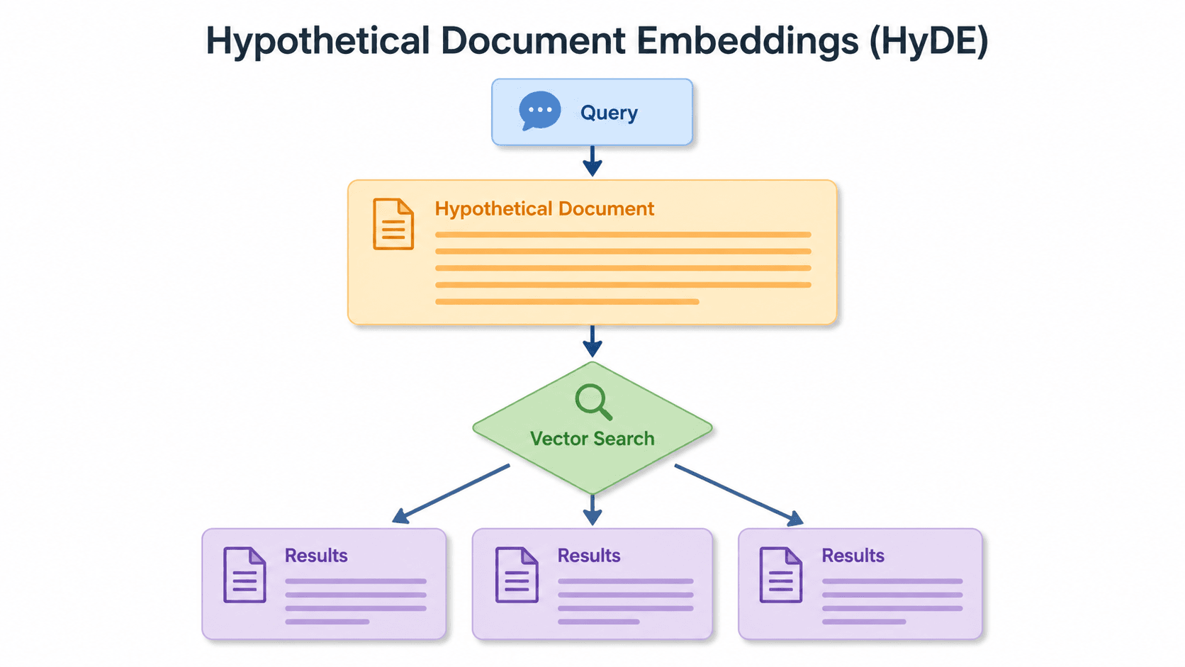
Short queries, formal documents: how HyDE improved semantic search precision by 50% in Elasticsearch
HyDE boosts semantic search precision and recall by 50% on short queries. Here's how to implement it in Elasticsearch with the Inference API and semantic_text.
June 24, 2026
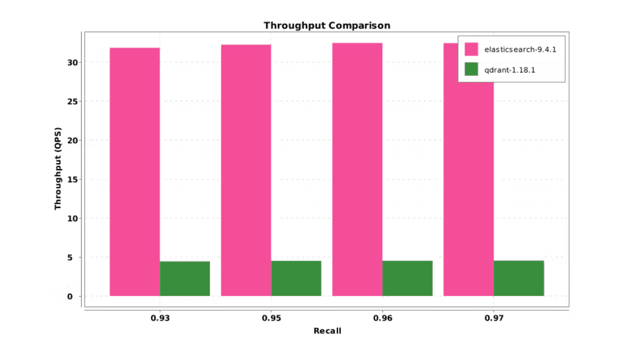
Elasticsearch DiskBBQ delivers 7x faster vector search than Qdrant on network-attached storage
Elasticsearch DiskBBQ achieves up to 7x higher vector search throughput than Qdrant at comparable recall on network-attached storage. Explore the benchmark methodology and full results.
July 6, 2026
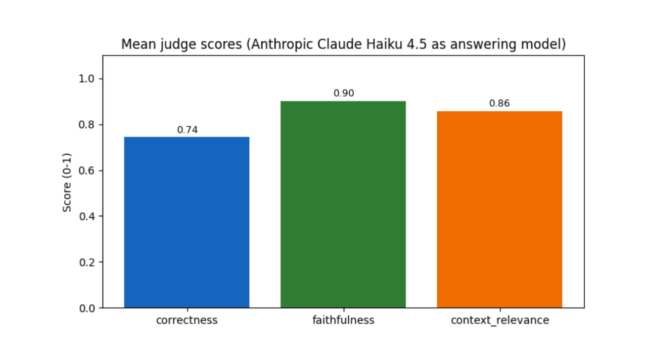
Who grades the grader? LLM-as-a-Judge inside Elasticsearch Workflows
Find out if your RAG agent is ready to ship. Score it on correctness, faithfulness and retrieval quality using only Elasticsearch Workflows and two Claude models.

June 15, 2026
Your search index is already an agent memory system: Persistent agent memory for Claude Code with Elasticsearch
Give your AI agent persistent cross-session memory using Elasticsearch: Hybrid recall, a knowledge graph, and cross-device handoffs. Three commands to install.

June 15, 2026
Your FAQ bot doesn't need a PhD: LLM query routing with Elastic Workflows
Route LLM queries by complexity using Elasticsearch search metadata: Mistral Small for FAQ questions, Claude Sonnet for multi-source synthesis.