Finding your best music friend with vectors: Spotify Wrapped, part 5

In the first part we talked about how to retrieve your Spotify data and visualize it. In the second part we talked about how to process the data and how to visualize it. In the third part we explored anomaly detection and how it helps us find interesting listening behavior. The fourth part uncovered relationships between the artists by using Kibana Graph. In this part, we talk about how to use vectors to find your music friend.

Discover your musical friends with vectors

A vector is a mathematical entity that has both magnitude (size) and direction. In this context, vectors are used to represent data, such as the number of songs listened to by a user for each artist. The magnitude corresponds to the count of songs played for an artist, while the direction is determined by the relative proportions of the counts for all artists within the vector. Although the direction is not explicitly set or visualized, it is implicitly defined by the values in the vector and their relationships to one another.

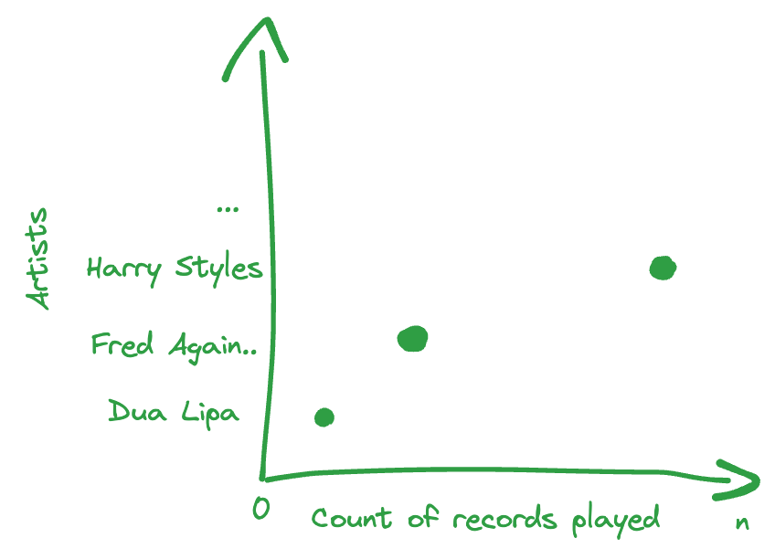
The idea is to simply create a huge array where we do a key => value sorting approach. The key is the artist and the value is the count of listened to songs. This is a very simple approach and can be done with a few lines of code. We create this vector:

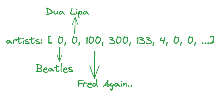
Which is super interesting because it is now sorted by the artist name. This gives us zero values for all artists we didn't listen to, or which the user didn't even know existed.

Finding your musical match then becomes a straightforward task of calculating the distance between two vectors and identifying the closest match. Several methods can be used for this, such as the dot product, euclidean distance, and cosine similarity. Each method behaves differently and may yield varying results. It is important to experiment and determine which approach best suits your needs.

How does cosine similarity, Euclidian distance and dot product work?

We will not delve into the mathematical details of each method, but we will provide a brief overview of how they work. To simplify, let’s break this down into just two dimensions: Ariana Grande and Taylor Swift. User A listens to 100 songs by Taylor Swift, user B listens to 300 songs by Ariana Grande, and user C falls in the middle, listening to 100 songs by Taylor Swift and 100 songs by Ariana Grande.

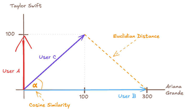
• The Cosine Similarity is better the smaller the angle and focuses on the direction of the vectors, ignoring their magnitude. In our case, user C will match with user A and user B equally because the angle between their vectors is the same (both are 45^\circ).

• The Euclidian distance measures the direct distance between two points, with shorter distances indicating higher similarity. This method is sensitive to both direction and magnitude. In our case, user C is closer to user A than to user B because the difference in their positions results in a shorter distance.

• The dot product calculates similarity by summing the products of the corresponding entries of two vectors. This method is sensitive to both magnitude and alignment. For example, user A and user B result in a dot product of 0 because they have no overlap in preferences. User C matches more strongly with user B (300 × 100 = 30,000) than with user A (100 × 100 = 10,000) due to the larger magnitude of user B’s vector. This highlights the dot product’s sensitivity to scale, which can skew results when magnitudes differ significantly.

In our specific use case, the magnitude of the vectors should not significantly impact the similarity results. This highlights the importance of applying normalization (more on that later) before using methods like Euclidean distance or dot product to ensure that comparisons are not skewed by differences in scale.

Data distribution

The distribution of our dataset is a crucial factor, as it will play a significant role later when we work on finding your best musical match.

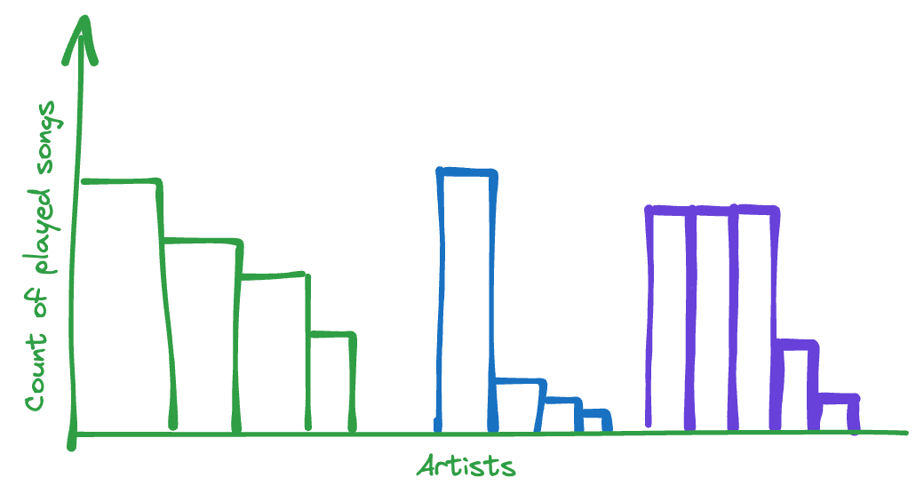
More details about the diversity of the dataset are discussed in the subheading Dataset Issues within the dense_vector section. The primary issue lies in the distribution of listened-to artists for each user. Each color represents a different user, and we can observe various listening styles: some users listen to a wide range of artists evenly distributed, while others focus on just a handful, a single artist, or a small group. These variations highlight the importance of considering user listening patterns when creating your vector.

Using dense_vector type

First of all, we created the vector above already, now we can store that in a field of dense_vector. We will auto create the dimensions we need in the Python code, based on our vector length.

elasticsearch.indices.create(
    index="spotify-dense-vector",
    mappings={
        "properties": {
            "artists": {
                "type": "dense_vector",
                "dims": len(unique_artists)
            },
            "user": {
                "type": "keyword"
            }
        }
    },
)

Whoops that errored in our case with this message: Error: BadRequestError(400, 'mapper_parsing_exception', 'The number of dimensions should be in the range [1, 4096] but was [33806]'): Ok, so that means our vector artists is too large. It is 33806 items long. Now, that is interesting, and we need to find a way to reduce that. This number 33806 represents the cardinality of artists. Cardinality is another term for uniqueness. It is the number of unique values in a dataset. In our case, it is the number of unique artists across all users.

One of the easiest ways is to rework the vector. Let's focus on the top 1000 commonly used artists. This will reduce the vector size to exactly 1000. We can always increase it to 4096 and see if there is something else going on then.

GET spotify-history/_search?size=0
{
  "aggs": {
    "user": {
      "terms": {
        "field": "user"
      },
      "aggs": {
        "artists": {
          "terms": {
            "field": "artist",
            "size": 1000
          }
        }
      }
    }
  }
}

This method of aggregation gives us the top 1000 artists per user. However, this can lead to issues. For instance, if there are 7 users and none of the top 1000 artists overlap, we end up with a vector dimension of 7000. When testing this approach, we encountered the following error: Error: BadRequestError(400, 'mapper_parsing_exception', 'The number of dimensions should be in the range [1, 4096] but was [4456]'). This indicates that our vector dimensions were too large.

To resolve this, there are several options. One straightforward approach is to reduce the top 1000 artists to 950, 900, 800, and so on until we fit within the 4096 dimension limit. Reducing the top n artists per user to fit within the 4,096-dimension limit may temporarily resolve the issue, but the risk of exceeding the limit will resurface each time new users are added, as their unique top artists will increase the overall vector dimensions. This makes it an unsustainable long-term solution for scaling the system. We already sense that we will need to find a different solution.

GET spotify-history/_search?size=0
{
  "aggs": {
    "artists": {
      "terms": {
        "field": "artist",
        "size": 1000
      },
      "aggs": {
        "user": {
          "terms": {
            "field": "user"
          }
        }
      }
    }
  }
}

Dataset issues

We adjusted the aggregation method by switching from calculating the top 1000 artists per user to calculating the overall top 1000 artists and then splitting the results by user. This ensures the vector is exactly 1000 artists long. However, this adjustment does not address a significant issue in our dataset: it is heavily biased toward certain artists, and a single user can disproportionately influence the results.

As shown earlier, Philipp contributes roughly 35% of all data, heavily skewing the results. This could result in a situation where smaller contributors, like Chris, have their top artists excluded from the top 1000 terms or even the 4096 terms in a larger vector. Additionally, outliers like Stefanie, who might listen repeatedly to a single artist, can further distort the results.

To illustrate this, we converted the JSON response into a table for better readability.

It is immediately apparent that there is an issue with the dataset. For example, Casper and K.I.Z, both German artists, appear in the top 5, but Casper is overwhelmingly influenced by Stefanie, who accounts for approximately 99% of all tracks listened to for this artist. This heavy bias places Casper at the top spot, even though it might not be representative across the dataset.

To address this issue while still using the 4096 artists in a dense vector, we can apply some data manipulation techniques. For instance, we could consider using the diversified_sampler or methods like softmax to calculate the relative importance of each artist. However, if we aim to avoid heavy data manipulation, we can take a different approach by using a sparse_vector instead.

Using a sparse_vector type

We tried squeezing our vector where each position represented an artist into a dense_vector field, however it's not the best fit as you can tell. We are limited to 4096 artists and we end up with a large array that has a lot of null values. Philipp might never listen to Pink Floyd yet in the dense vector approach, Pink Floyd will take up one position with a 0. Essentially, we were using a dense vector format for data that is inherently sparse. Fortunately, Elasticsearch supports sparse vector representation through the sparse_vector type. Let’s explore how it works!

{
  "artists": {
    "Casper": 1334,
    "Fred again..": 22561,
    "Ariana Grande": 10234
  }
}

Instead of creating one large array, we will create a key => value pair and store the artists name next to the listened count. This is a much more efficient way of storing the data and will allow us to store a higher cardinality. There is no real limit to how many key value pairs you can have inside the sparse_vector. At some point the performance will degrade, but that is a discussion for another day. Any null pairs will simply be skipped.

What does a search look like? We take the entire content of artists and put that inside the query_vector and we use the sparse_vector query type and only retrieve the user and the score.

GET spotify-sparse-vector-total_count/_search
{
  "fields": [
    "user"
  ],
  "query": {
    "sparse_vector": {
      "field": "artists",
      "query_vector": {
        "Fred again..": 4096
        "Ariana Grande": 3508,
        "Harry Styles": 2535,
        ...
      }
    }
  }
}

Normalization

Using a sparse_vector allows us to store data more efficiently and handle higher cardinality without hitting the dimension limit. The tradeoff, however, is that we are limited to using the dot product for similarity calculations, which means we cannot directly use methods such as cosine similarity or Euclidean distance. As we saw earlier, the dot product is heavily influenced by the amplitude of vectors. To minimize or avoid this effect, we will first need to normalize our data.

We provide the full sparse vector to identify our “music best friend.” This straightforward approach has yielded some interesting results, as shown here. However, we are still encountering a similar issue as before: the influence of vector magnitudes. While the impact is less severe compared to the dense_vector approach, the distribution of the dataset still creates imbalances. For example, Philipp might match disproportionately with many users simply due to the vast number of artists he listens to.

This raises an important question: does it matter if you listen to an artist 100, 500, 10,000, or 25,000 times? The answer is no—it’s the relative distribution of preferences that matters. To address this, we can normalize the data using a normalizing function like Softmax, which transforms raw values into probabilities. It exponentiates each value and divides it by the sum of the exponentials of all values, ensuring that all outputs are scaled between 0 and 1 and sum to 1.

You can normalize directly in Elasticsearch using the normalize aggregation or programmatically in Python using Numpy. With this normalization step, each user is represented by a single document containing a list of artists and their normalized values. The resulting document in Elasticsearch looks like this:

{
  "user": "philipp",
  "artists": {
    "Fred again..": 0.013858094401620936,
    "Ariana Grande": 0.0073373738573697155,
    "Harry Styles": 0.002186232187442565,
    "Too Many Zooz": 0.0019208388258044266,
    "Kraftklub": 0.001862001480735705,
    "Jamie xx": 0.0015681941691341277,
    "Billy Talent": 0.001156093556076037,
    "Billie Eilish": 0.0008427954862422548,
    "Lizzo": 0.000744181016015583,
    ...
  }
}

Finding your music match is rather easy. We take the entire document for the user Philipp since we want to match him against everyone else. The search looks like this:

GET spotify-sparse-vector-softmax/_search
{
  "fields": [
    "user"
  ],
  "query": {
    "sparse_vector": {
      "field": "artists",
      "query_vector": {
        "Fred again..": 0.013858094401620936,
        "Ariana Grande": 0.0073373738573697155,
        "Harry Styles": 0.002186232187442565,
        "Too Many Zooz": 0.0019208388258044266,
        "Kraftklub": 0.001862001480735705,
        "Jamie xx": 0.0015681941691341277,
        "Billy Talent": 0.001156093556076037,
        ...
      }
    }
  }
}

The response is in JSON and contains the score and the user; we altered it to a table for better readability, then the score is multiplied by 1.000 to remove leading zeros.

On an untuned and out of the box softmax we see that Philipp's best friend is Karolina with a score of 0.050... followed relatively closely by Stefanie with 0.049.... Emil is furthest away from Philipp's taste. After comparing the data for Karolina and Philipp (using the dashboard from the second blog), this seems a bit odd. Let's explore how the score is calculated. The issue is that in untuned softmax, the top artist can get a value near 1 and the second artist is already on 0.001..., which emphasises your top artist even more. This is important because the dot product calculation used to identify your closest match works like this:

Karolina: Dua Lipa: 1
Philipp: Dua Lipa: 0.33

When we calculate the dot product we do 1 * 0.33 = 0.33, which boosts my compatibility with Karolina a lot. When Philipp is not matching on the top artist of anyone else with a higher value than 0.33, Karolina is my best friend, even though we might have barely anything else in common. To illustrate this here is a table of our top 5 artists, side by side. The number represents the spot in the top artists.

We can observe that Philipp overlaps with Karolina's top 5 artists. Even though they range from place 15, 32, 119, 126, 378 for Philipp, any value that Karolina has is multiplied by Philipp's ranking. In this case, the order of Karolina's top artists weighs more than Philipp's. There are a few ways to fix softmax by adjusting temperature and smoothness. Just trialing out some numbers for temperature and smoothness, we end up with this result (score multiplied by 1.000 to remove leading zeros). A higher temperature describes how sharply softmax assigns the probabilities, this distributes the data more evenly, whilst a lower temperature emphasises a few dominant values, with a sharp decline.

Adding the temperature and smoothness altered the result. Instead of Karolina being Philipp's best match, it moved to Stefanie. It's interesting to see how adjusting the method of calculating the importance of an artist heavily impacts the search.

There are many other options available for building the values for the artists. We can look at the total percentage of an artist represented in a dataset per user. This could lead to better distribution of values than softmax and ensure that the dot product, like described above with Karolina and Philipp for Dua Lipa, wouldn't be that significant anymore. One other option would be to take the total listening time into consideration and not just the count of songs, or their percentage. This would help with artists that publish longer songs that are above ~5-6 minutes. One Fred Again.. a song might be around 2:30 and that would allow Philipp to listen to twice as many songs as someone else. The listened_to_ms is in milliseconds and we end up with a similar discussion around, if a sum() is the correct approach, similar to count of songs played. It is an absolute number, where the higher it gets, the less importance the higher number should get accounted for. We could account for listening completion, there is a listened_to_pct and we could pre-filter the data to only songs that our users finish to at least 80%. Why bother with songs that are skipped in the first few seconds or minutes? The listening percentage punishes people that listen to a lot of songs from random artists using the daily recommended playlists, whilst it emphasises those who like to listen to the same artists over and over again. There are many many opportunities to tweak and alter the dataset to get the best results. All of them take time and have different drawbacks.

Conclusion

In this blog we took you with us on our journey to identify your music friend. We started off with a limited know-how of Elasticsearch and thought that dense vectors are the answers, and that lead to looking into our dataset and diverting to sparse vectors. Along the way we looked into a few optimisations on the search quality and how to reduce any sort of bias. And then we figured out a way that works best for us and that is the sparse vector with the percentages. Sparse vectors are what powers ELSER as well; instead of artists, it is words.