Custom Vega Visualizations in Kibana 6.2
Interested in a walkthrough of Vega-based visualizations in Kibana? Check out this video.
Beginning with Kibana 6.2, users can now go beyond the built-in visualizations offered. This new visualization type lets users create custom visualizations without developing their own plugin using an open source JSON-based declarative language called Vega, or its simpler version called Vega-Lite.
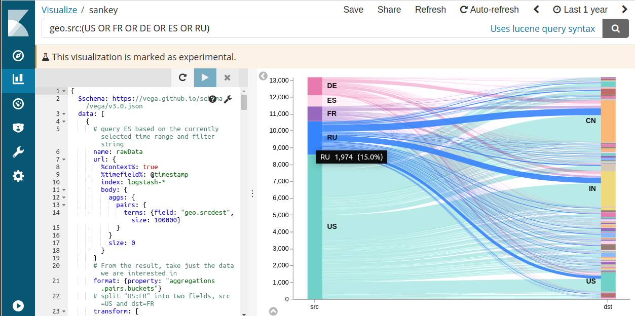
Unlike other visualizations, the Vega vis is a blank canvas on which you, the developer, can draw visual elements based on one or more data sources including custom URLs. For example, you can design a Sankey diagram of the network traffic patterns. This Sankey visualization will be demonstrated in the next blog post.
Hello World Scatter Plot with Vega-Lite
Our first example will be drawing a scatter plot from the sample Logstash data using the simpler Vega-Lite language.
Data
The first step of any Vega visualization is to get the right data using Elasticsearch query language. We will use 3 fields from the sample Logstash data. The data was generated using makelogs utility. This query can be tried in the “dev tools” tab to see the full result structure. We will use the same query as part of the Vega code below.
GET logstash-*/_search
{
  "size": 10,
  "_source": ["@timestamp", "bytes", "extension"]
}
The output is an array of these elements inside the { hits: { hits: [...] }} structure:
{ "hits": { "hits": [
  {
    "@timestamp": "2018-02-01T18:05:55.363Z",
    "bytes": 2602,
    "extension": "jpg"
  },
  ...
] }}
Drawing
Now create a new Vega visualization. If the Vega vis is not listed, ensure lab visualizations in advanced settings (visualize:enableLabs) are enabled. Delete the default code, and paste this instead. Vega vis is written using JSON superset called HJSON.
{
$schema: https://vega.github.io/schema/vega-lite/v2.json
data: {
# URL object is a context-aware query to Elasticsearch
url: {
# The %-enclosed keys are handled by Kibana to modify the query
# before it gets sent to Elasticsearch. Context is the search
# filter as shown above the dashboard. Timefield uses the value
# of the time picker from the upper right corner.
%context%: true
%timefield%: @timestamp
index: logstash-*
body: {
size: 10000
_source: ["@timestamp", "bytes", "extension"]
}
}
# We only need the content of hits.hits array
format: {property: "hits.hits"}
}
# Parse timestamp into a javascript date value
transform: [
{calculate: "toDate(datum._source['@timestamp'])", as: "time"}
]
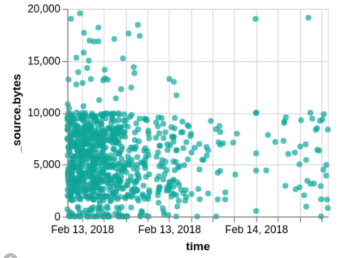
# Draw a circle, with x being the time field, and y - number of bytes
mark: circle
encoding: {
x: {field: "time", type: "temporal"}
y: {field: "_source.bytes", type: "quantitative"}
}
}
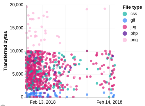
We should make a few more cleanups and improvements:
- Disable X axis title by adding axis: { title: null } to x encoding
- Set Y axis title with axis: { title: "Transferred bytes" }
- Make dots different color and shape depending on the extension field: add this to encodings:
color: {field:"_source.extension", type:"nominal", legend: {title:"File type"}}
shape: {field:"_source.extension", type:"nominal"}
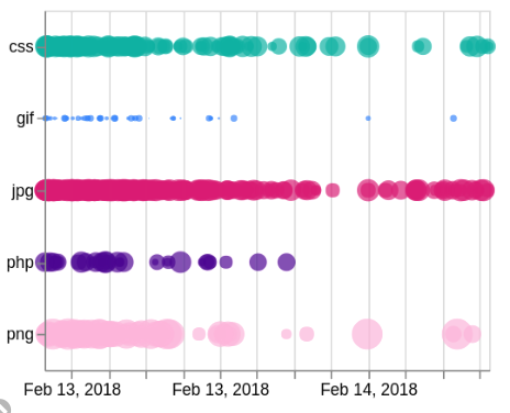
We could even change the visualization entirely by putting extension as the y axis, and using size. Replace all of encodings with these:
x: {field: "time", type: "temporal", axis: {title: null}}
y: {field: "_source.extension", type: "nominal", axis: {title: null}}
size: {field: "_source.bytes", type: "quantitative", legend: null}
color: {field: "_source.extension", type: "nominal", legend: null}
Building Trend Indicator with Vega
For the Vega example, let’s build a very simple trend indicator to compare the number of events in the last 10 minutes vs the 10 minutes before that.
We can ask Elasticsearch for the 10 min aggregates, but those aggregates would be aligned on 10 minute boundaries, rather than being the “last 10 minutes”. Instead, we will ask for the last 20 aggregates, 1 minute each, excluding the current (incomplete) minute. The extended_bounds param ensures that even when there is no data, we still get a count=0 result for each bucket. Try running this query in the Dev Tools tab - copy/paste it, and hit the green play button.
GET logstash-*/_search
{
  "aggs": {
    "time_buckets": {
      "date_histogram": {
        "field": "@timestamp",
        "interval": "1m",
        "extended_bounds": { "min": "now-20m/m", "max": "now-1m/m" }
      }
    }
  },
  "query": {
    "range": {
      "@timestamp": { "gte": "now-20m/m", "lte": "now-1m/m" }
    }
  },
  "size": 0
}
The result would be
{
  // ... skipping some meta information ...
  "aggregations": {
    "time_buckets": {
      "buckets": [
        {
          "key_as_string": "2018-02-09T00:52:00.000Z",
          "key": 1518137520000,
          "doc_count": 1
        },
        {
          "key_as_string": "2018-02-09T00:53:00.000Z",
          "key": 1518137580000,
          "doc_count": 3
        },
        // ... 18 more objects
    ]
  }
}
And the actual Vega spec with inline comments:
{
  # Schema indicates that this is Vega code
  $schema: https://vega.github.io/schema/vega/v3.0.json
  # All our data sources are listed in this section
  data: [
    {
      name: values
      # when url is an object, it is treated as an Elasticsearch query
      url: {
        index: logstash-*
        body: {
          aggs: {
            time_buckets: {
              date_histogram: {
                field: @timestamp
                interval: 1m
                extended_bounds: {min: "now-20m/m", max: "now-1m/m"}
              }
            }
          }
          query: {
            range: {
              @timestamp: {gte: "now-20m/m", lte: "now-1m/m"}
            }
          }
          size: 0
        }
      }
      # We only need a specific array of values from the response
      format: {property: "aggregations.time_buckets.buckets"}
      # Perform these transformations on each of the 20 values from ES
      transform: [
        # Add "row_number" field to each value -- 1..20
        {
          type: window
          ops: ["row_number"]
          as: ["row_number"]
        }
        # Break results into 2 groups, group #0 with row_number 1..10,
        # and group #1 with row numbers being 11..20
        {type: "formula", expr: "floor((datum.row_number-1)/10)", as: "group"}
        # Group 20 values into an array of two elements, one for
        # each group, and sum up the doc_count fields as "count"
        {
          type: aggregate
          groupby: ["group"]
          ops: ["sum"]
          fields: ["doc_count"]
          as: ["count"]
        }
        # At this point "values" data source should look like this:
        # [ {group:0, count: nnn}, {group:1, count: nnn} ]
        # Check this with F12 or Cmd+Opt+I (browser developer tools),
        # and run this in console:
        #   console.table(VEGA_DEBUG.view.data('values'))
      ]
    }
    {
      # Here we create an artificial dataset with just a single empty object
      name: results
      values: [
        {}
      ]
      # we use transforms to add various dynamic values to the single object
      transform: [
        # from the 'values' dataset above, get the first count as "last",
        # and the one before that as "prev" fields.
        {type: "formula", expr: "data('values')[0].count", as: "last"}
        {type: "formula", expr: "data('values')[1].count", as: "prev"}
        # Set two boolean fields "up" and "down" to simplify drawing
        {type: "formula", expr: "datum.last>datum.prev", as: "up"}
        {type: "formula", expr: "datum.last<datum.prev", as: "down"}
        # Calculate the change as percentage, with special handling of 0
        {
          type: formula
          expr: "if(datum.last==0, if(datum.prev==0,0,-1), (datum.last-datum.prev)/datum.last)"
          as: percentChange
        }
        # Calculate which symbol to show - up or down arrow, or a no-change dot
        {
          type: formula
          expr: if(datum.up,'🠹',if(datum.down,'🠻','🢝'))
          as: symbol
        }
      ]
    }
  ]
  # Marks is a list of all drawing elements.
  # For this graph we only need a single text mark.
  marks: [
    {
      type: text
      # Text mark executes once for each of the values in the results,
      # but results has just one value in it. We could have also used it
      # to draw a list of values.
      from: {data: "results"}
      encode: {
        update: {
          # Combine the symbol, last value, and the formatted percentage
          # change into a string
          text: {
            signal: "datum.symbol + ' ' + datum.last + ' ('+ format(datum.percentChange, '+.1%') + ')'"
          }
          # decide which color to use, depending on the value
          # being up, down, or unchanged
          fill: {
            signal: if(datum.up, '#00ff00', if(datum.down, '#ff0000', '#0000ff'))
          }
          # positioning the text in the center of the window
          align: {value: "center"}
          baseline: {value: "middle"}
          xc: {signal: "width/2"}
          yc: {signal: "height/2"}
          # Make the size of the font adjust with the size of the visualization
          fontSize: {signal: "min(width/10, height)/1.3"}
        }
      }
    }
  ]
}
This is the first of many for the Vega blog post series! Be on the lookout for our next post where we’ll create a Sankey chart. And make sure to check out this video walkthrough of Kibana visualizations with Vega.