BKD-backed geo_shapes in Elasticsearch: precision + efficiency + speed
With the addition of new data structures in Lucene 6.0, the Elasticsearch 5.0 release delivered massive indexing and search performance improvements for one-dimension numeric, date, and IP fields, and two-dimension (lat, lon) geo_point fields. Building on this work, the Elasticsearch 6.0 release further improved usability and simplicity of the geo_point API by setting the default indexing structure to the new block k-d tree (BKD) and removing all support for legacy prefix tree encoding. Starting with Elasticsearch 7.0, we are excited to present the details of the new default indexing technique for geo_shape field types that, once again, delivers an immense performance improvement over the legacy prefix tree indexing approach for geospatial geometries. With the improvements described here, geo_shape fields created in 7.0 and later guarantee 1 cm accuracy while, on average, providing faster searching and several times faster indexing compared to 6.x geo shapes
The need for a new approach
For the past several years the geo_shape mapping parameters have been a source of confusion and frustration for many users. Finding the right configuration parameters to strike a balance between spatial accuracy and index / search performance often demanded an unreasonable amount of effort and understanding of the inner data structures from our users. In some cases users either gave up or were unable to find an acceptable configuration and were stuck with poor performance. For a company that strives for simplicity for our users and demands a high level of performance from our products, we wanted to do better. Building on past efforts, we set out to provide a similar level of performance improvement with geo_shape that we achieved with geo_point.

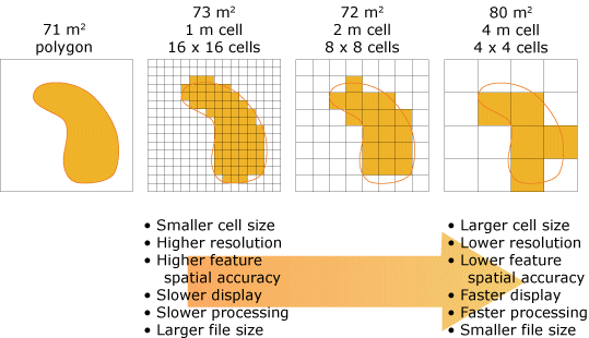
Until the release of the BKD tree, the inverted index was the only data structure available for providing search capabilities. This structure, originally intended for searching text documents, relied on converting unstructured text into a stream of tokens. This can be thought of as splitting sentences into a stream of words. To use this structure for spatial indexing, Lucene needed a way to convert the spatial geometries into a stream of tokens representing the coverage area. This was achieved through a technique known as rasterization; a process that converts line graphics into a stream of cells. For images and graphics displays, each cell is the equivalent of a pixel which has a fixed size. Search applications, on the other hand, strive to store the most amount of data with the smallest index possible, so fixed size spatial cells are not required. In fact, storing all cells at a fixed size causes an unnecessarily large index. For geospatial geometries, the size of the cell translates to a square size on the earth’s surface; this is known as spatial resolution (represented as tree_levels or precision in the mappings). The following image (source: ESRI) illustrates the trade-offs that need to be considered when selecting an appropriate spatial resolution.
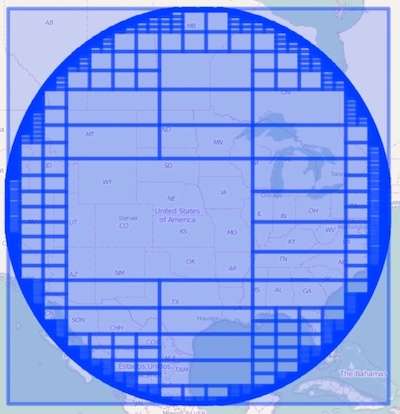
To achieve organized structure with an efficient storage footprint the spatial index employed the use of quadtrees; a hierarchical organization of cells where each cell is recursively partitioned into quadrants. This eliminates the need to store all cells by only recursing to the highest resolution for cells that fall on the boundary of the geometry. The following image illustrates a point radius circle decomposed into a hierarchical set of cells using Lucene’s quadtree implementation (note the highest resolution and sheer number of cells on the boundary of the circle). Each cell is then encoded into a morton code (binary representation) so it can be inserted into the inverted index. In addition to the spatial resolution issues (including the search accuracy problem where all points and geometries inside the smallest cell need to be linearly scanned at query time) converting a single vector geometry into a stream of raster cells introduces an index size overhead proportional to the size of the shape; the larger the shape the larger the index.
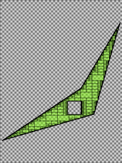
It’s clear that while this approach works, it carries a number of drawbacks that quickly become realized with even the simplest of shapes. The following image illustrates an eight vertex polygon covering a 1 degree by 1 degree square latitude, longitude area. Using the quadtree approach, with spatial resolution set to 3 meters, results in 1,105,889 terms in the inverted index; and that’s just for one shape! From this example It’s clear the cost of using a rasterized index necessitated a new, more efficient, approach to indexing and searching spatial geometries at massive scale.
Inspired by computer graphics...
Dealing with high resolution geometries, level of detail, and limitations in graphics computing performance is not a unique or novel problem. Remaining in vector space and avoiding the conversion of vector geometries to cell based rasters was the first realization to overhauling and improving the shape indexing in Lucene. By remaining in vector space we avoid many of the spatial resolution issues encountered when indexing in raster space. To efficiently store and display high resolution geometries, most computer graphics and game engines decompose these geometries into primitives, such as triangles. Triangles are largely efficient because, “every object can be split into triangles but a triangle cannot be split into anything else than triangles”. The following image (source: Arm® Technologies) illustrates two different geometry resolutions displayed as a collection of triangles.
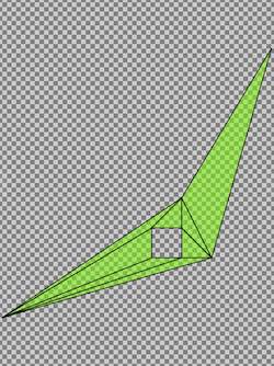
To achieve this, we needed an efficient triangular tessellation algorithm that converts input vector geometry into a stream of triangles that remain in vector space. We turned to David Eberly’s 2002 paper, “Triangulation by Ear Clipping” and quickly found that our friends at Mapbox had adapted the same algorithm to their WebGL rendering layer in an implementation they call earcut. This reputability was encouraging and we quickly adapted a similar approach and benchmarked its performance against the original quadtree implementation. The following image illustrates one of those benchmarks. Using the same simple eight vertex polygon as demonstrated above, covering a 1 degree by 1 degree square latitude, longitude area the triangular tessellation approach was applied. After a 7 ms computation performance (in a development environment, so your mileage may vary) the polygon was decomposed into a total of eight triangle terms versus 1,105,889 quad terms using the rasterization approach used in prefix tree indexing. This represents a 138,236 to 1 compression ratio! Keeping the geometry in vector space also means we no longer have to worry about the spatial resolution issues associated with the quad cells; so geometries nearly remain in the same resolution as provided by the user. More on this below.
Encoding and indexing…
With triangular tessellation, the number of terms have been significantly reduced and the original accuracy of the geometry has been maintained, but geometries are now represented as a collection of triangles instead of their original vertex form. With this change the shape indexing and search problem is reduced to a process of organizing the triangles into the BKD data structure such that search is efficient. Achieving this required two additional improvements.
First, the BKD data structure needed a way to optimally organize the triangular geometries. This was achieved through a modification of the BKD implementation referred to as selective indexing. The objective with selective indexing is to allow N-dimensional fields to designate the first k dimensions (index dimensions) for driving the construction of the BKD tree with the remaining d dimensions (data dimensions) as stored ancillary data for use at the leaf nodes. For the collection of 2D triangles, the first four dimensions were chosen as index dimensions representing the bounding box of the triangle. By doing this, the general BKD tree is converted into an R-tree where the internal nodes of the tree are a collection of bounding boxes, and the leaves contain data required to reconstruct the original triangles.
The second improvement needed was a compact dimensional encoding of the individual tessellated triangles such that they could be stored efficiently at the leaves of the tree without requiring an unnecessarily large amount of space. This was accomplished using three data dimensions (seven total dimensions) that enable the encoding to reconstruct the three 2D vertices of the triangle from the first four bounding box dimensions. However, in order to support all spatial relations (e.g., CONTAINS queries when the original indexed geometries are no longer maintained) the following requirements are needed:
- Triangle vertices must be encoded in counter-clockwise orientation.
- Triangle vertex order can start at any point; e.g., triangle ABC satisfies the following relationship: ABC == CAB == BCA
These two assumptions enable an efficient encoding where original triangles can be reconstructed in such a way that orientation is preserved while being able to mark which triangle edge belongs to the original geometry. The following image illustrates the eight possible encodings for tessellated triangles.
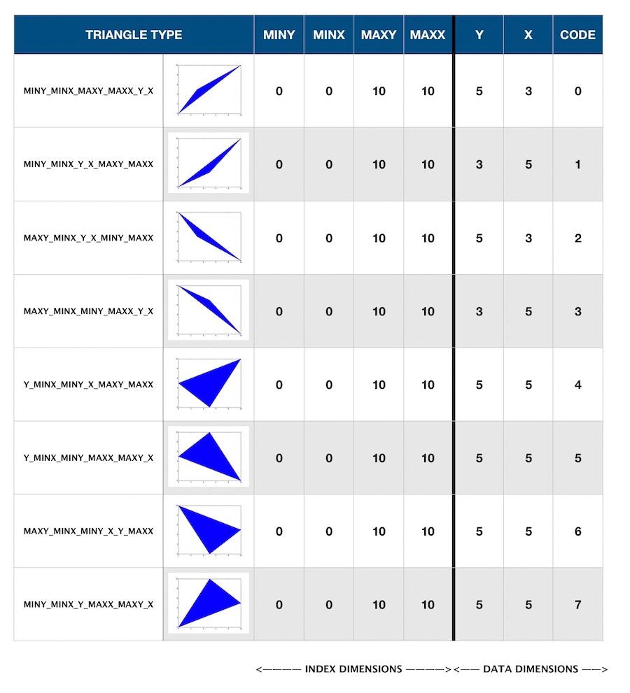
In the chart above, the “code” dimension indicates which vertex(es) are shared with the original bounding box and how to reconstruct the remaining vertex(es) from the min/max bounding box index dimensions and y, x data dimensions. In the first row, for example, the code dimension ‘0’ indicates the triangle shares the (Ymin, Xmin), and (Ymax, Xmax) vertices with the bounding box index dimensions. The third triangle vertex can then be reconstructed using the Y and X data dimensions directly. With this encoding, the tessellated triangles are efficiently indexed using a total of seven dimensions such that the BKD data structure is organized as an R Tree that is optimal for spatial search while being able to reconstruct the original vertices of the triangle from a small amount of ancillary data.
Finally, to keep the index size as small as possible, each dimensional value is passed through a quantization function that converts from 64-bit double precision floating point to a 32-bit integer space. This process enables better compression of the stored triangles and bounding boxes resulting in an index that is more than half the size of storing the original values. It is important to note, however, that the quantization function is slightly lossy and introduces a spatial error of 1 cm. This means precision of the original geometry is no longer maintained but will be guaranteed within 1 cm accuracy.
Performance benchmarks and more resources
While we plan to cover other performance improvements, BKD optimizations, benchmarks, new features, and changes in future blog posts, Mike McCandless maintains a series of limited nightly Lucene benchmarks that can be followed while more optimizations are made to the internal data structures. Keep in mind that all benchmark configurations vary and no one single benchmark is perfect so, as always, your mileage may vary. Of course the Lucene community would love to hear any feedback you may have and if you run into any issues with the Elastic stack feel free to reach out on the Elastic Discuss forums. Thank you and we look forward to further improving and enhancing your spatial search experience!