Explaining the Bucket Span in Machine Learning for Elasticsearch
Editor's Note (August 3, 2021): This post uses deprecated features. Please reference the map custom regions with reverse geocoding documentation for current instructions.
With the release of the Elastic Stack 5.5, machine learning (ML) is now a supported GA version. Along with this, we have introduced an experimental feature which allows the end-user to estimate the bucket span for an anomaly detection job. This is available when using the single or multi metric job creation wizards, but not when using the advanced configuration wizard.
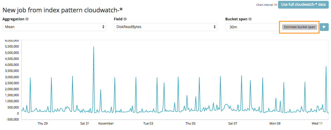
The bucket span estimator gives you the minimum viable bucket span based on the characteristics of a pre-viewed subset of your data. It’s a useful starting point for your analysis. However, once comfortable with the concepts of anomaly detection, then we urge you to delve a little deeper and make sure you have the right bucket span for your use case and your needs.
Typically in our experience for machine data, bucket spans tend to be between 10 minutes and 1 hour, but it depends on the characteristics of the data.
To explain more about bucket spans, and how to configure this appropriately, let me answer a few commonly asked questions.
What is a bucket span?
When analyzing data, we use the concept of a bucket to divide up a continuous stream of data into batches for processing.
For example, if you were monitoring the average response time of a system, using a bucket span of 1 hour means that at the end of each hour we would calculate the average (mean) value of the last hour’s worth of data and compute the anomalousness of that average value compared to previous hours.
Figure 1 shows a comparison of bucketed and non-bucketed data.
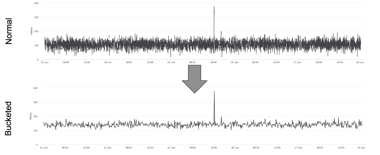
By analyzing the data in buckets, we can more easily see significant changes, random fluctuations are smoothed, and there is a discrete range to model.
As the time series data is gathered into buckets this also reduces the bandwidth and space required to process and store the data. This is important for online anomaly detection, especially in large scale environments.
Why is the bucket span important?
In machine learning terms, the bucket span and function define the feature we model. Choosing a shorter bucket span allows anomalies to be detected more quickly but at the risk of being too sensitive to natural variations or noise in the input data. Choosing too long a bucket span can mean that interesting anomalies are smoothed out.
Figure 2 shows what the same data can look like when viewed at three different bucket spans. This chart plots the sum of a counter over time with coloured vertical lines denoting detected anomalies; light blue is a warning, dark blue a minor, orange a major and red a critical anomaly.
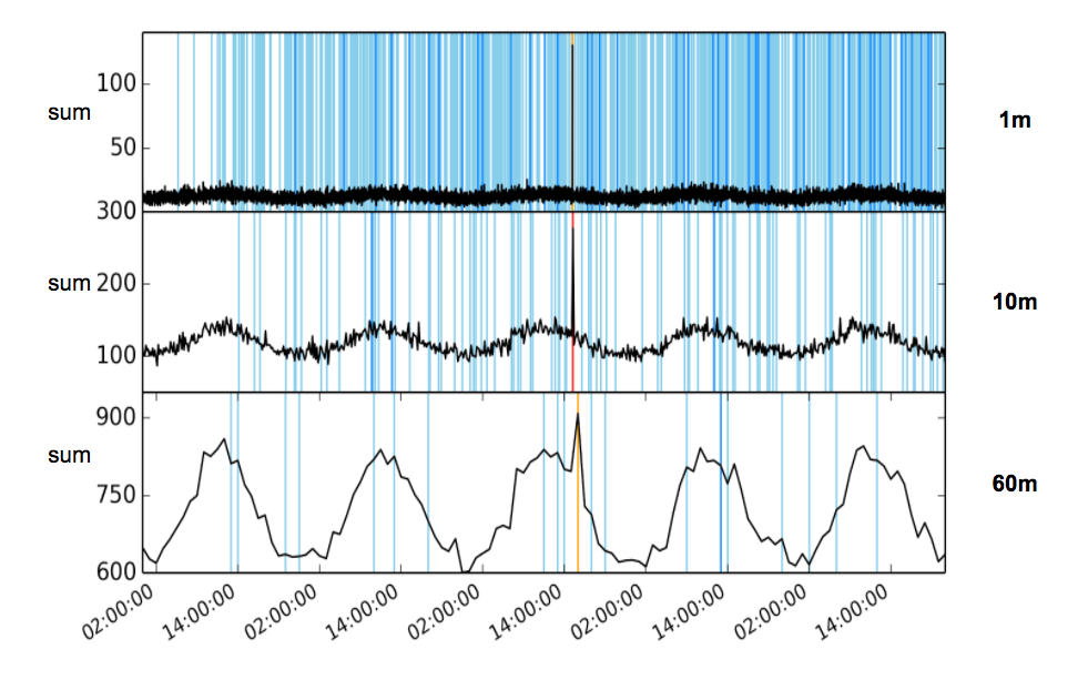
In the top most chart, a bucket span of 1 minute has been selected. This is as fine as the data rate, and the fluctuations in the data give rise to a very high background noise of anomalies. The periodic trend is not particularly visible.
In the bottom chart, a bucket span of 1 hour has been selected. We can clearly see that the trend becomes significantly more visible with respect to the noise as a larger bucketing interval is used. However, there are noticeably fewer anomalies.
Part of this reduction is due to the fact that anomalies are now only calculated hourly. However some anomalies have been hidden in the mass of data that exists in a larger bucket. Notice that the single important anomaly has a lower severity, and is only considered “major” rather than “critical”. For this data using the sum function, the use of a larger bucket has meant that the relative importance of the anomaly has been reduced in significance.
In this example for this dataset, choosing a bucket span of 10 minutes provides an optimal balance of granularity, time to alert and prominence of the anomaly.
How does the bucket span affect the time to alert?
One might infer that (on average) an anomaly will be reported at least half a bucket span away from when it occurred. This is not true, but there are some caveats which depend on the job configuration and the characteristics of your data.
Assuming you are using a datafeed to pass data from Elasticsearch indices to ML for analysis, a search is performed every frequency for new data since the last received timestamp. The default value for frequency is adjusted depending on the bucket span.
| Bucket Span | Default frequency |
| Less than 2 minutes | 1 minute |
| Less than 20 minutes | bucket_span
|
| Less than or equal to 12 hours | 10 minutes |
| More than 12 hours | 1 hour |
Data is analyzed in time-order, so once a data point is received for the next bucket, end-of-bucket processing is triggered and the analysis moves forward in time. End-of-bucket processing applies the latest bucket summary statistics to the model and calculates the final results for this bucket (amongst other things).
As we receive interim data when using a datafeed, we also calculate interim results at the frequency interval. Interim results make adjustments for the fact that only partial data has been seen for the bucket. For functions such as min and max, interim results are very reliable. For functions such as sum, mean and count, then the reliability depends on the characteristics of the data. Adjustments for partial buckets with continuous data can be very accurate. However if your data time stamps are irregular and low volume, then it becomes difficult to assess how much of the bucket has been seen so confidence is less and interim anomalies may not be found (or in the case of low_count or low_sum functions may be inaccurate).
So by default for a 1-hour bucket span, interim results are calculated every 10 minute and alerts can occur at this granularity. This blog post describes how to implement alerting on ML jobs in more detail.
Interim results are short lived, and are only available for the latest partial bucket. Once end-of-bucket processing has occurred, they are updated as final results.
There is an overhead to calculating interim results, so setting the frequency value too low will negatively impact the performance of the system.
How does the bucket span estimator work?
The bucket span estimator is available when creating a job using the single metric or multi metric job creation wizard.
It performs a series of tests on a subset of data, taken from the previous 250 hours from the end date in the Kibana time picker.
First, it checks if the data is polled. This is data that is stored at discrete time intervals, for example monitoring data that is reported every 5 mins would be polled data. If the data is polled, we estimate the bucket span such that at least one data point exists per bucket,
If the data is not considered to be polled, we then created multiple aggregated time series for a set of bucket spans (from 5 minutes to 3 hours) using the aggregation function that has been selected in the detector configuration.
If the job is multi metric, then there may be more than one detector and many entities. The aggregation described above is performed for every detector function and for a selection of 10 entities using a partitioned search.
It then performs a series of tests on each aggregated time series, starting with the smallest bucket span. The estimated bucket span is the smallest span for which all tests have passed.
- Empty bucket test - at least 20% of buckets must be populated
- Minimum doc count test - for functions sum and count, at least 5 documents are required per bucket
- Scale variation test - if a trend exists, the smoothing effect of bucketing does not hide this trend when compared to a longer reference span
For multi metric jobs, the results are reduced by taking the median value of partitioned series per detector and then the median of the detector series to get a single value.
If the bucket span cannot be estimated, a warning message will be displayed and the bucket span should be manually entered. Consider the factors below in choosing a bucket span as a span shorter than 3 hours may still be appropriate.
What do I need to consider when choosing the bucket span?
It is important to note that the estimated bucket span is only a rough calculation, based on the subset of data seen. It does not take into account other operational factors such as time to alert, the typical duration of anomalies, and the processing time. As such you may wish to choose your own span.
Selecting the optimal bucket span can be a compromise across multiple factors discussed below:
Data Characteristics - In order to get enough data in each bucket we have to take into account if the data is sparse or if the data is polled. Sparse data typically requires a longer bucket span or use of a sparse-aware function e.g. non_null_sum or non_zero_count. Polled data requires at least one data point per bucket.
Quality and Relevance - In general we want to maximise the anomaly detection rate and minimise the false positives. To do this we should match the bucket span to be similar to the typical duration of interesting anomalies. This requires knowledge of the system beforehand, which may not always be available.
Performance - The main computation is performed at the end of each bucket, known as end-of-bucket processing. With a longer bucket span we can achieve higher data throughput compared with a shorter bucket span. If end-of-bucket processing takes longer than the bucket span, then the job will not be able to keep up with real-time. In this instance, selecting a longer bucket span allows the processing time to catch up.
Timeliness - End-of-bucket processing will finalize results for the most recent bucket. If your data is not suited to interim results and the job is time critical, then you may wish to reduce the bucket span.
Why can’t I change the bucket span?
Once the analysis is underway, we do not allow configuration changes to the bucket span. Changing the bucket span would fundamentally change what data is being modelled. Summary statistics that had been gathered for the life of the job up to this point, would no longer be applicable to future data. The analysis would need to start gathering these summary statistics from scratch, and thus the model would be reset.
As the model would be starting from zero again, then we feel it is preferably to do this as a new job. This job could be run on the same historical data to start with and then progress in real-time. The advantage of doing this would be that you could see the two job results in parallel. By comparing the results, you can then decide which bucket span provided the most informative and actionable results for your environment.