Seamlessly connect with leading AI and machine learning platforms. Start a free cloud trial to explore Elastic’s gen AI capabilities or try it on your machine now.
On almost every large Elastic deployment I’ve worked with, there’s an Elastic Security or Elastic Observability anomaly detection (AD) job that looks healthy but is perpetually behind. Six hours behind. Twelve. And the gap never closes.
The datafeed isn’t broken. It’s doing exactly what it was built to do: reading every raw document, across every shard, every run. On a large cluster with cross-cluster search (CCS) and a broad index pattern, like logs-*, that means scanning billions of documents per bucket. There’s no hardware that makes that sustainable. The datafeed will always be chasing live data and never reaching it.
The fix is to switch from the default scroll-based datafeed configuration to an aggregation-based datafeed configuration: Let the data nodes summarize locally, and ship only compact bucket results to the ML node. Same detections, a fraction of the load. The speedup can be dramatic. More than you might expect. The numbers are in the next section. The explanation for why the gap is so large is at the end of the post, for those who want to understand the mechanics.
One catch worth knowing now: Switching requires creating a new job. The old model doesn’t transfer; weeks of learned baseline are lost. The right time to make this switch is before the job has been running for months, not after. That’s the main reason to read this before you deploy.
How much faster? Scroll vs. aggregation datafeeds for ML jobs
We ran the same job two ways on production data: first scroll-based, and then aggregation-based. The job covered 13 months of history, monitoring 836,000 log events per hour in 15-minute buckets across multiple clusters.
Training on historical data with scroll-based configuration: five days of wall-clock time, 7.9 million sequential requests, and 3.5 TB transferred; with aggregations: 2.3 minutes, 23 requests, and 34 MB (a 3,374× speedup). Think of it this way: If you start the scroll backfill at 9 a.m. Monday, it will finish Saturday morning. The aggregation version is done by 9:02 a.m.
On live data, the difference is less dramatic but still meaningful: around 20× fewer requests per tick. That adds up quickly when the datafeed runs every few minutes around the clock.
Before you start
Three things worth knowing before diving into the configuration.
This isn't wizard territory. The standard Kibana job wizards (Single Metric, Multi-Metric, Population) don't expose aggregation configuration. To create an aggregation-based job, you need either the Elasticsearch API or Kibana's Advanced Job Wizard, with JSON edited by hand. The worked example below shows the most practical path: Configure the job in the Multi-Metric Wizard, and then click Convert to advanced job before creating it. That gets you a prefilled JSON starting point instead of a blank editor.
The configuration is unforgiving and mostly silent about it. There's no schema validation that catches a misnamed aggregation key or a fixed_interval that doesn't match bucket_span. The job will run, anomalies will fire, and nothing will indicate that the results are based on the wrong data. This is why the five-step pattern exists and why the Preview tab is worth using every time: Catching a misconfiguration before the job trains is a 30-second check; catching it a week later is a much worse afternoon.
The Single Metric Viewer has a known limitation with aggregated jobs. That viewer reconstructs the "actual" data curve by re-querying the index, but it can't reproduce an arbitrary, user-defined aggregation, so the actual-value line is typically missing or approximate. The Anomaly Explorer is unaffected: Anomaly scores, swim lanes, and influencer attribution all work normally. Just don't rely on the Single Metric Viewer's chart for visual validation of what the model saw.
What we can and can’t aggregate
Almost every ML function works with aggregated datafeeds, but the right aggregation pattern depends on the function.
| Function | Pattern |
|---|---|
| `count`, `mean`, `high_mean`, `low_mean`, `sum`, `max`, `min` | Standard: `date_histogram` → `terms` → metric aggregation |
| `time_of_day`, `time_of_week` | Minimal: plain `date_histogram`, no `terms` or metric needed |
| `rare`, `freq_rare`, `info_content` | Composite: top-level composite with `date_histogram` as a source |
| `categorization` | `terms` on the `.keyword` subfield of the categorization field |
| `lat_long`, `varp` | Scroll only |
lat_long and varp are the genuine exceptions. If you want to use these detectors, you are required to use the scroll-based datafeed configuration.
The five-step pattern in the next section covers the standard case. We’ll walk through the remaining patterns at the end of the post.
The standard five-step pattern: Scroll-based to aggregation datafeed
Converting any scroll-based job to an aggregation-based datafeed follows the same five steps. Once you understand the pattern, applying it to any compatible job takes about 10 minutes.
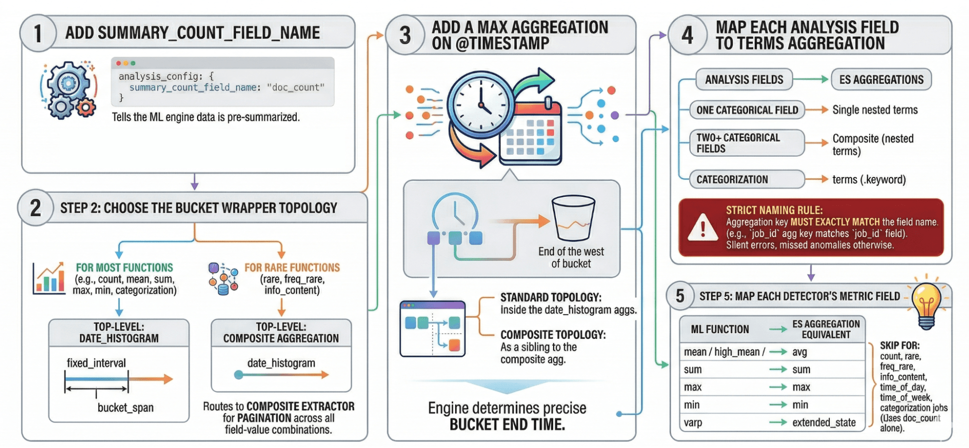
Step 1: Add summary_count_field_name: "doc_count" to the analysis config. This tells the ML engine that incoming data is pre-summarized. Without it, the engine treats each aggregated bucket as a single raw document and produces wrong anomaly scores.
Step 2: Choose the bucket wrapper topology. For most functions (count, mean, sum, max, min, varp, time_of_day, time_of_week, and categorization) use a date_histogram at the top level whose fixed_interval matches your bucket_span exactly to ensure accurate analysis. For rare, freq_rare, and info_content, use a composite at the top level with a date_histogram as one of its sources. This routes the datafeed to the composite extractor, which paginates through all field-value combinations rather than truncating to a top-N.
Step 3: Add a max aggregation on @timestamp. The ML engine needs this to determine the precise end time of each bucket. In the standard topology (Step 2, date_histogram outer), it goes inside the histogram’s aggregations. In the composite topology, it sits as a sibling of the composite aggregation.
Step 4: Map each analysis field to a terms aggregation, named exactly after the corresponding field in the analysis config. One categorical field → a single nested terms. Two or more categorical fields → a composite aggregation nested inside the date_histogram, with one terms source per field. For categorization jobs, use a terms aggregation on the .keyword subfield of the categorization_field_name. The naming rule is strict: The aggregation key must exactly match the field name in the analysis config; the ML engine uses the aggregation name, not the field parameter, to look up values. A mismatch produces silently wrong results; no error, just a job that appears to run while missing everything meaningful.
Step 5: Map each detector’s metric field to its Elasticsearch aggregation equivalent:
| ML function | Elasticsearch aggregation |
|---|---|
| `mean` / `high_mean` / `low_mean` | `avg` |
| `sum` | `sum` |
| `max` | `max` |
| `min` | `min` |
For count, rare, freq_rare, info_content, time_of_day, time_of_week, and categorization jobs, the ML engine works from doc_count alone; no metric aggregation is needed, and this step can be skipped.
Step-by-step example: Building an aggregation-based ML job in Kibana
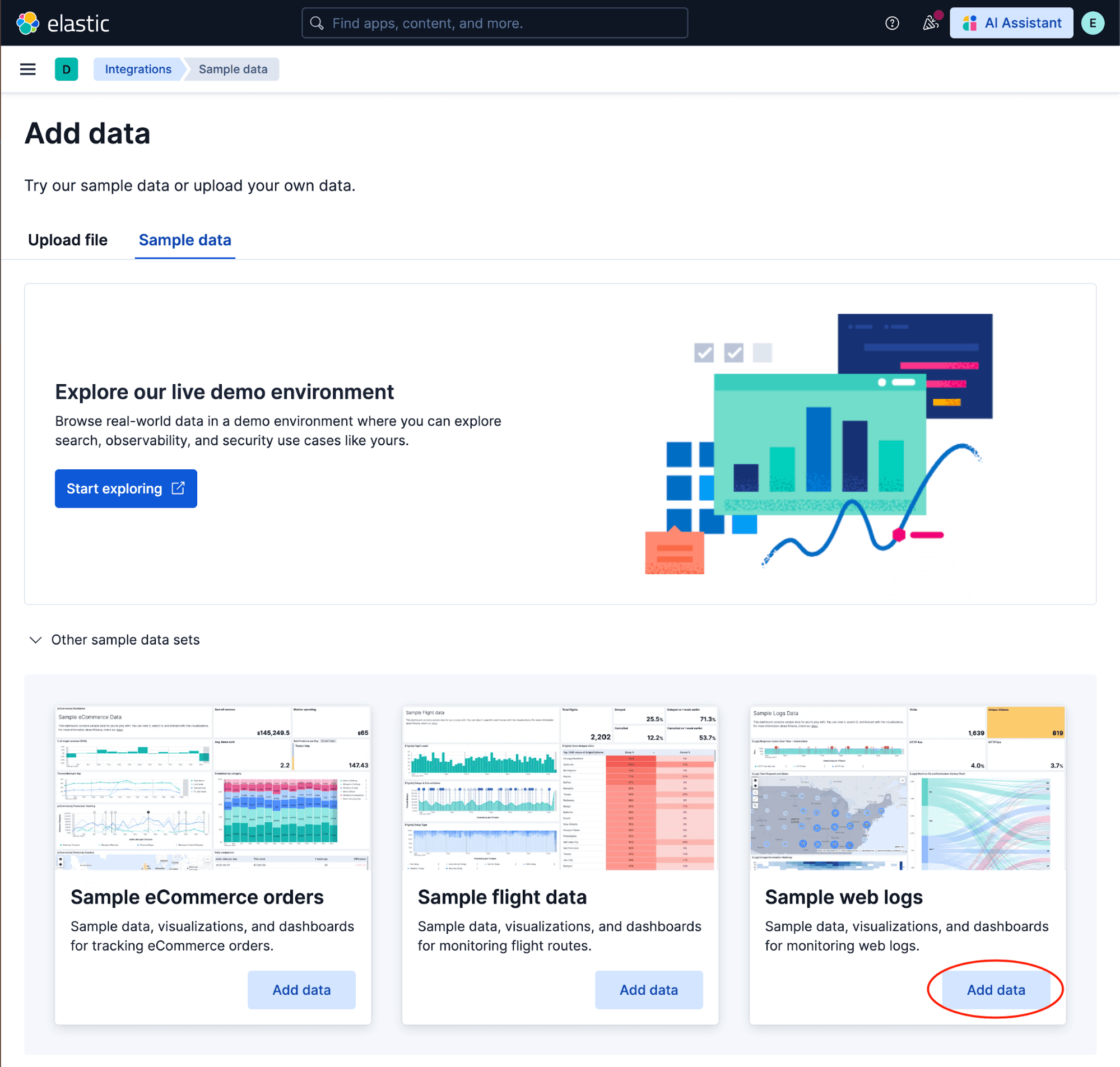
Let’s build this end to end using Kibana’s sample web logs. If you haven’t loaded them yet, go to the Kibana home page and click Integrations → Sample data → Sample web logs → Add data. This gives us a data view called Kibana Sample Data Logs and an index called kibana_sample_data_logs with fields including @timestamp, bytes (response size), and geo.dest (destination country).
We’ll build a job that detects unusually large response sizes: high_mean of bytes, partitioned by destination country (geo.dest), with a 1-hour bucket span.
Creating the job with the Multi-Metric Wizard
This is how most jobs get created in practice. Navigate to Machine Learning → Anomaly Detection → Manage Jobs → Create job.
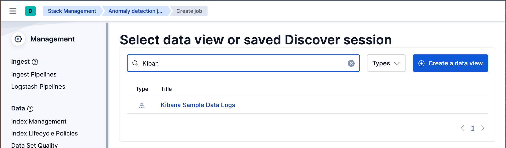
Select the “Kibana Sample Data Logs” data view, and set the time range to cover the full sample dataset. On the job type screen, choose Multi-metric.
In the Multi-Metric Wizard, configure the detector:
- High mean of
bytes. - Split data by
geo.dest. - Bucket span:
1h.
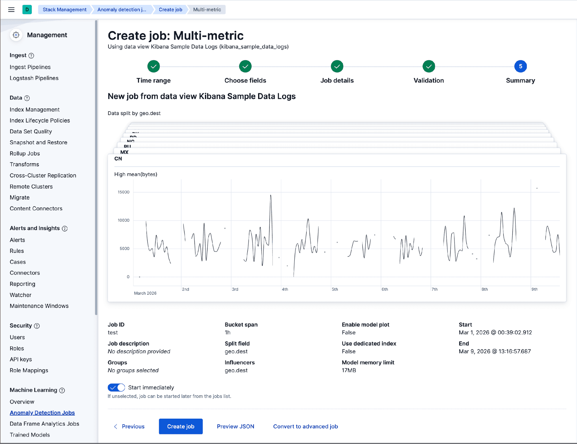
Give the job an ID, and leave everything else at its defaults, but don’t click Create yet. On this last configuration step, click on Preview JSON and look at the datafeed section. What you’ll see is a plain scroll-based datafeed with no aggregations, just an index pattern and a match_all query.
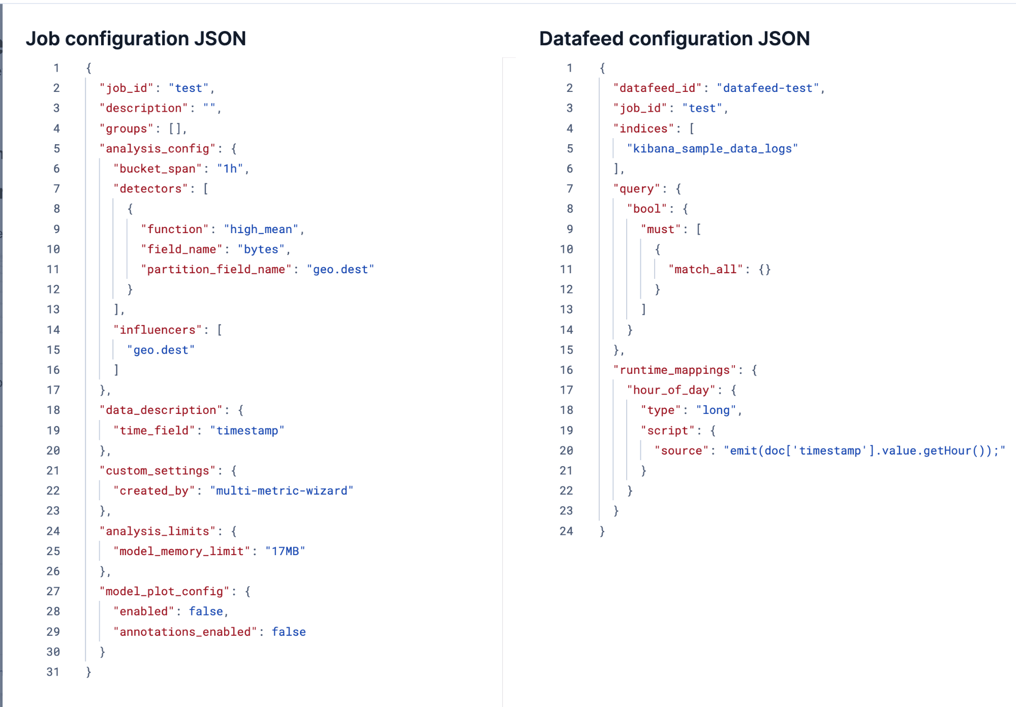
This is the default every wizard produces. On a small cluster, it works fine. On a large cluster with CCS and a broad index pattern, this datafeed will scan every raw document on every run and never catch up with live data.
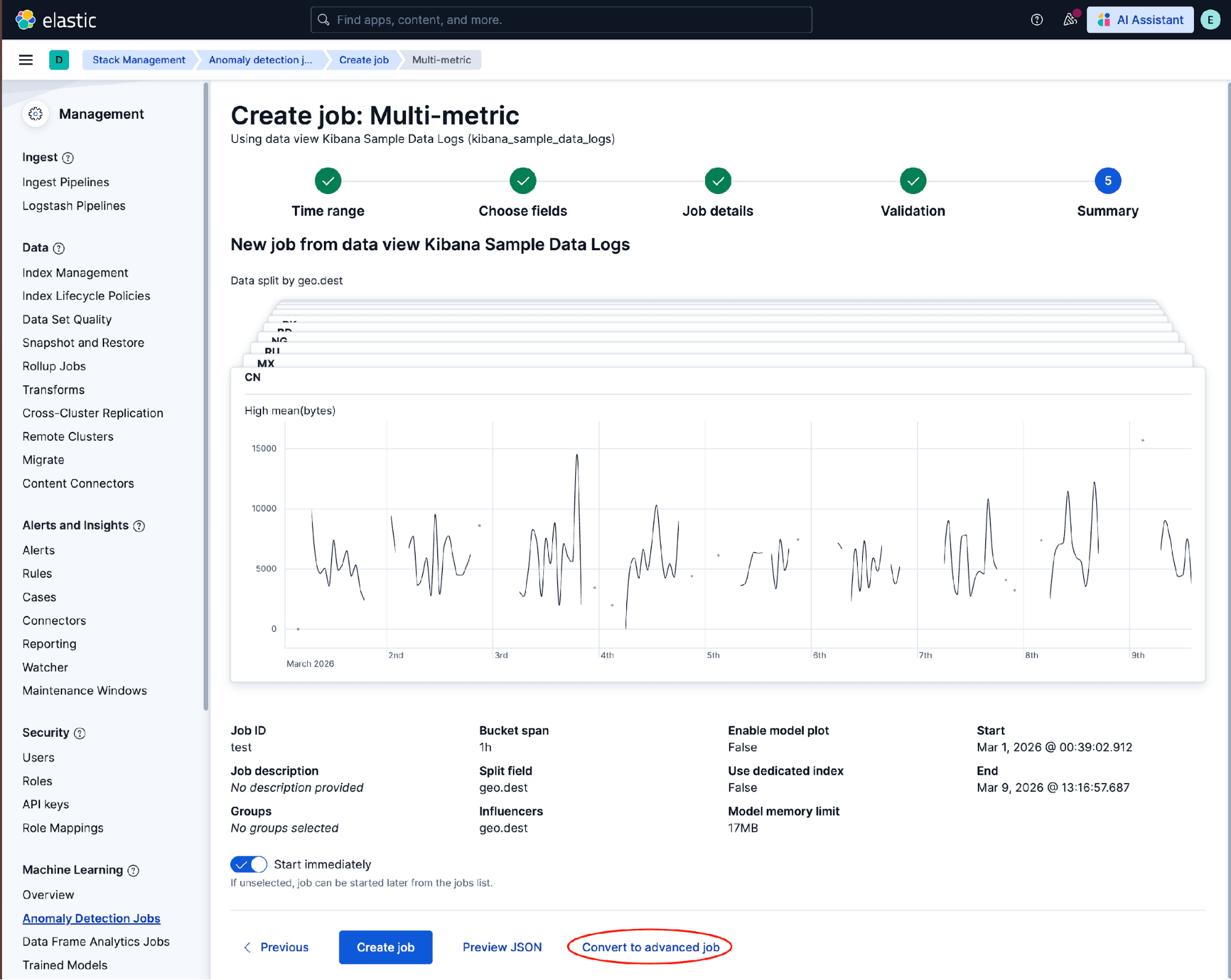
Instead of clicking Create, click Convert to advanced job. This keeps everything you just configured (the detector, the partition field, the bucket span) and drops you directly into the Advanced Wizard, where we can apply the five-step pattern.
Analysis configuration
The conversion prefills the detector, partition field, and bucket span. The only change needed here is Step 1 of the pattern: Open the Edit JSON view, and add summary_count_field_name to tell the ML engine that incoming data will be pre-summarized:
Datafeed configuration
Switch to the Datafeed tab. This is where Steps 2 through 5 of the pattern come together. Remove scroll_size if it’s present, and then enter the aggregations:
A few notes on this config:
- Step 2: The
date_histogramusesfixed_interval:"1h", matchingbucket_spanexactly. A mismatch produces incorrect bucket timing. - Step 3: The
maxaggregation on@timestampmust be named@timestampand placed inside the histogram’saggregations; without it, the ML node can’t determine the precise end of each bucket. - Step 4: The
termsaggregation for the partition field must be named exactly after the partition field:geo.dest, notgeo.dest_groupingor any alias. The ML engine uses the aggregation name, not thefieldparameter, to identify which partition value each bucket belongs to. A mismatch silently drops the partition field from results entirely. - Step 5: The metric aggregation key
bytesmatchesfield_namein the detector exactly. Any mismatch here produces silently wrong anomaly scores.
Validate with the preview
Before we create the job, let’s use the Preview tab. This runs the aggregation against real data and shows exactly what the ML node will receive, a very useful sanity check before committing.
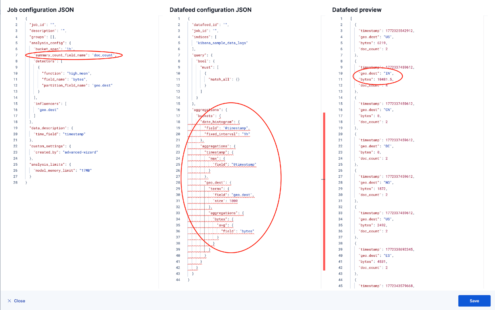
Three things to verify in the preview output: doc_count should be present on every bucket and greater than 1. The bytes values should look like average response sizes: numbers in the hundreds to hundreds of thousands for web traffic. And each row should correspond to a distinct (timestamp, geo.dest) pair. If anything looks off, fix it in the JSON editor and rerun the preview.
Adding influencer fields
In the example above, geo.dest is the partition field. The ML model learns a separate baseline for each destination country, and anomalies are reported per country. But you might also want machine.os to appear as an influencer in anomaly results: When the detector fires, you want to see “this looks anomalous for geo.dest: CN and machine.os: win is a contributing factor.” Influencers don’t drive anomaly detection; they provide context for the anomalies that are found.
To support an influencer alongside a partition field, the analysis config gains an influencers array:
And now the datafeed needs to aggregate on both fields simultaneously. One terms nested inside another terms won’t work; a nested terms surfaces only the top-N values of the inner field per outer bucket, so you’d silently lose combinations. Instead, use a composite aggregation with one terms source per field, next to the date_histogram:
composite generates one bucket per unique (geo.dest, machine.os) combination. The ML node sees every pair and can correctly attribute which operating system was contributing when a country’s response sizes spiked. Use the preview to confirm distinct pairs appear. If you only see a handful of rows where you’d expect many, the size parameter on the composite may need to be raised.
Categorization
Categorization works with aggregated datafeeds: summary_count_field_name and categorization_field_name can coexist in the same job. The five-step pattern applies directly. Step 2 uses the standard date_histogram topology. Step 4 has one adjustment: Instead of a partition field, we aggregate the text field itself using a terms aggregation on its .keyword subfield, named to match categorization_field_name exactly. Step 5 is skipped. The count detector works from doc_count alone.
Analysis config:
Datafeed aggregations:
The datafeed sends one bucket per unique message.keyword value with a doc_count for each. The ML node receives those strings, runs categorization on them, assigning an mlcategory to each, and the count detector tracks how many documents fall into each category per bucket. The naming rule from Step 4 applies: The terms aggregation must be named message, matching categorization_field_name in the analysis config exactly.
One thing to watch: Keyword fields have a default ignore_above: 256 limit. Log messages longer than 256 characters won’t be indexed as .keyword and will be silently excluded from the aggregation. If your log messages are long, check the field mapping before using this approach. You may need to raise the limit in your index template.
The minimal pattern for
time_of_day and time_of_week are the easiest functions to aggregate: They only need a timestamp and a document count. The C++ process extracts the time component from the bucket timestamp and builds a cyclical model of normal activity; doc_count tells it how many events fell in each bucket. No terms sources, no metric aggregation, no composite.
Analysis config:
Datafeed aggregations:
A plain date_histogram is enough; no composite needed. This makes time_of_day and time_of_week particularly CCS-friendly: one request per time chunk, minimal data over the wire. Use the same structure for time_of_week; only the function name changes.
If you want to add a partition_field_name (for example, to model time-of-day patterns per service), add a terms aggregation inside the histogram’s aggregations following the standard Step 4 pattern.
The composite pattern for
rare, freq_rare, and info_content all need the composite extractor, the one that paginates through all unique value combinations rather than truncating to top-N. The five-step pattern applies here with a different topology in Step 2: composite goes at the top level (not date_histogram), with date_histogram as a source inside it. Step 3 places the max @timestamp aggregation as a sibling of the composite, and Step 5 is skipped since all three functions work from doc_count alone.
The datafeed structure is the same for all three functions: a composite at the top level, a date_histogram as one of its sources, and one terms source per analysis field. The only thing that varies is which fields you include as terms sources: rare needs one source for by_field_name; freq_rare needs sources for both by_field_name and over_field_name; info_content needs a source for field_name plus any by_field_name or over_field_name fields. None of the three require a metric aggregation.
A few notes:
- The composite aggregation must be the top-level aggregation, not nested inside a
date_histogram. This is what routes the datafeed to the composite extractor. - The
date_histogramis a source inside the composite, not the outer wrapper. Itsfixed_intervalmust divide evenly intobucket_span. - The
maxaggregation on@timestampsits as a sibling of thecomposite(insideaggregations), not nested inside it. composite.sizecontrols the page size per round trip. Setting it high (10000) reduces round trips, which matters with CCS latency. With three sources and high-cardinality fields, the total combination count can be large; the extractor paginates automatically.
Why aggregation-based datafeeds outperform scroll at scale
The gap is structural, not incidental. A scroll-based datafeed reads raw documents one page at a time: Every 1,000 documents is one request, and each waits for the previous one to complete before issuing the next. The number of requests is therefore proportional to the total document count in the time range being backfilled. At 836,000 events per hour over 13 months, that's roughly 7.9 billion events, or 7.9 million sequential round trips. Each round trip crosses the CCS boundary, waits for shard responses, and transfers matching documents in full. There’s no parallelism: The datafeed holds a scroll context open on the remote cluster and processes one page at a time.
An aggregation-based datafeed works differently. The data nodes summarize data locally, grouping by time bucket and categorical fields, and ship only the bucket results to the ML node. The number of requests is proportional to field cardinalities, not document count. In our example, two influencer fields with six unique combinations produce six result rows per time bucket; the datafeed pages through those in a handful of requests regardless of how many raw events fall in each bucket. Double the ingestion rate and the scroll request count doubles; the aggregation request count stays the same. This is why the gap widens at scale: The more data you have, the worse scroll looks by comparison, and the better aggregations look.
On live data, the picture is different because each real-time tick covers only one fresh bucket: Scroll issues however many pages fit in that bucket's worth of data, while aggregations issue one request. The 20× figure for live data reflects that ratio at 836,000 events per hour with a 15-minute bucket span. The practical threshold where aggregations stop being optional is when (ingestion rate × bucket span) > scroll_size; once a single bucket contains more than one scroll page of documents, the datafeed can't keep pace with live data regardless of hardware. Below that threshold, scroll is fine and aggregations are a nice-to-have. Above it, aggregations are the only sustainable option.
Scroll-based datafeeds are the right default, and the wizards make the right call for most deployments. At scale (more shards, broader index patterns, CCS across tiers), switching to an aggregation-based datafeed is the natural next step: The data nodes summarize where the data lives, the ML node processes compact results, and the detections stay the same. The one cost to know up front is model state: Switching requires a new job, so the earlier you make the move, the less you give up.
If you hit a case not covered here, an aggregation type that doesn’t map cleanly or a composite that behaves unexpectedly, the Elastic Discuss forums are a good place to continue.
Related Content
July 10, 2026
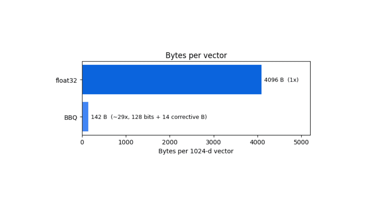
How BBQ shrinks Jina v5 embeddings by 29x without losing recall in Elasticsearch
A hands-on test comparing BBQ and float32 vector indices in Elasticsearch, measuring memory, disk and recall@10 across five languages.
July 21, 2026
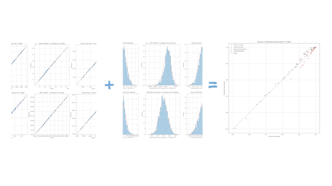
How Elasticsearch auto-tunes vector quantization to hit your recall target
Learn the geometric model that lets Elasticsearch predict recall with R² > 0.98 accuracy and auto-select vector quantization parameters from a small data sample.
June 24, 2026
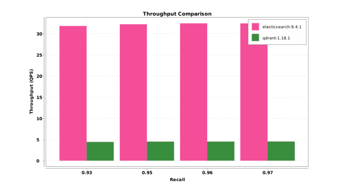
Elasticsearch DiskBBQ delivers 7x faster vector search than Qdrant on network-attached storage
Elasticsearch DiskBBQ achieves up to 7x higher vector search throughput than Qdrant at comparable recall on network-attached storage. Explore the benchmark methodology and full results.
July 24, 2026
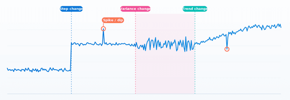
How Elasticsearch detects multiple change points in time series with 0.99 recall
ES|QL's CHANGE_POINT command finds structural shifts, variance changes and spikes in any metric in ~1ms, without tuning anything per series.
April 10, 2026
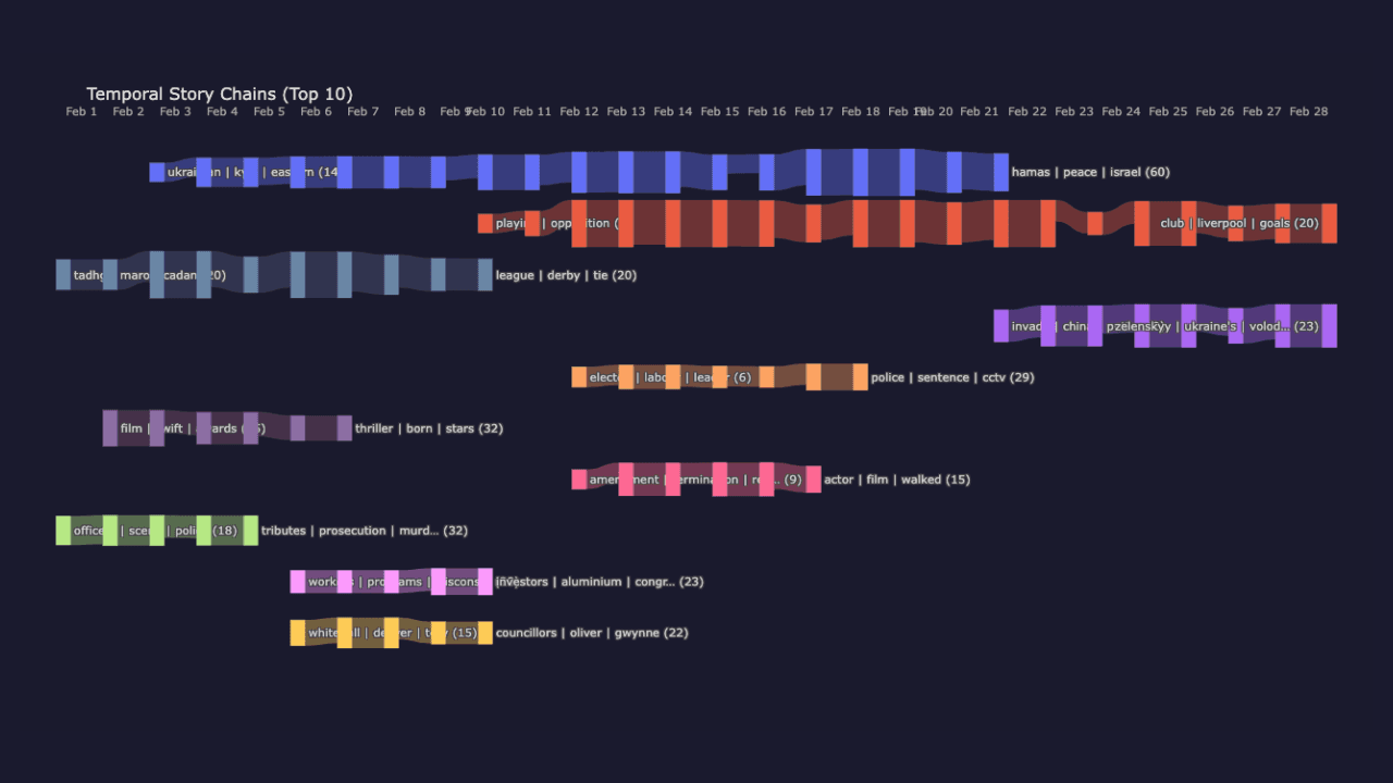
Unsupervised document clustering with Elasticsearch + Jina embeddings
A practical, reproducible approach to unsupervised document clustering with Elasticsearch and Jina embeddings.