From vector search to powerful REST APIs, Elasticsearch offers developers the most extensive search toolkit. Dive into our sample notebooks in the Elasticsearch Labs repo to try something new. You can also start your free trial or run Elasticsearch locally today.
NVIDIA cuVS builds HNSW graphs on the GPU, delivering up to 12x faster vector indexing in Elasticsearch. This post covers two production deployment patterns: Pattern A runs build and serve on the same GPU node, suited for clusters under five data nodes. Pattern B uses three lean GPU ingest nodes (64 GB RAM each) that hand off via ILM rollover to seven CPU hot-serving nodes (192 GB each) - the right default for production at scale. Full index template, ILM policy, and sizing math for a 300M-vector corpus are included.
What does the Elasticsearch cuVS GPU plugin actually do?
The Elasticsearch cuVS GPU plugin takes over HNSW graph construction during two operations: segment flush and force merge. The plugin requires a supported NVIDIA GPU attached to the data node, the cuVS plugin installed, and vectors.indexing.use_gpu: true in elasticsearch.yml.
- Segment flush. Vectors accumulate in the JVM write buffer. At flush, the plugin batches them, copies them to GPU VRAM via PCIe, constructs a CAGRA graph in VRAM, converts it to HNSW, copies the result back to system RAM via PCIe, and then Lucene writes the segment file to local NVMe. The segment is subsequently memory-mapped into the OS page cache for query serving.
- Force merge. When segments are merged, the same GPU path speeds up graph reconstruction, delivering approximately 7x faster force-merge times according to the published benchmark.
Everything else (HTTP request handling, query serving, cluster state management, ILM execution) runs on the CPU and uses system RAM. The GPU is a coprocessor for two write-path operations, not a replacement for the host compute environment.
The separation of GPU build from CPU query serving matters because GPU-attached nodes don't need to be the query-serving tier.They can be dedicated to the write path and hand off built shards to cheaper CPU hot-serving nodes. That's the core insight behind Pattern B.
Pattern A: combined GPU build and serve in one Elasticsearch node
Pattern A is the simpler deployment. Every GPU node builds shards and serves queries on those shards. This is how the cuVS benchmark was run: a single g6.4xlarge (64 GB RAM, 1x NVIDIA L4) running indexing on a single Elasticsearch process. The node is capable of both indexing and search concurrently, though the published benchmark measured indexing throughput specifically.
When to use combined GPU nodes (Pattern A)
- Small clusters (fewer than 5 data nodes).
- Proof-of-concept or edge deployments where operational simplicity outweighs cost optimization.
- Corpora small enough that the full HNSW graph fits in each node's page cache alongside normal operations.
Node configuration (Pattern A)
Every data node gets a GPU and the same elasticsearch.yml config:
No shard-routing tricks, no ILM tier separation. Shards land where Elasticsearch's default allocator puts them, and every node can both build and serve.
Note: there is also an index-level setting, index.vectors.indexing.use_gpu, that can override the node-level default on a per-index basis. Valid values are auto (default, uses GPU when available), true (requires GPU, fails if unavailable), and false (disables GPU for this index).
Sizing implications
Because each node holds long-lived shards, it needs enough system RAM for:
- JVM heap (~32 GB)
- OS page cache holding the HNSW graph for its share of the corpus
- OS and CUDA overhead (~10-15 GB)
For a 300M-vector int8 corpus with HA (two copies), each of 10 data nodes holds ~65 GB of HNSW data in page cache. Add JVM and overhead and you land at roughly 128–192 GB of system RAM per node. That's much more than the 64 GB reference benchmark because the benchmark held only 2.6M vectors on a single node.
System RAM per node scales with shards-per-node, not with total corpus size. More nodes at lower RAM, or fewer nodes at higher RAM. The tradeoff is operational complexity versus hardware cost.
A note on the published benchmark. The ~12x indexing throughput and ~7x force-merge numbers were measured using 2.6M vectors at 1,536 dimensions with float32 hnsw on a single g6.4xlarge node. This post's examples use 1,024 dimensions with int8_hnsw. Performance characteristics may vary with different dimension counts and quantization levels, so benchmark your own corpus for production sizing.
Pattern B: dedicated GPU ingest nodes with ILM shard handoff to CPU
Pattern B separates the cluster into two data tiers with different hardware profiles and different roles:
- GPU ingest tier. Small number of nodes with NVIDIA GPUs and modest system RAM (64 GB). These nodes accept writes, build HNSW segments on GPU via cuVS, and own the active write shard.
- CPU hot-serving tier. Larger number of nodes without GPUs and larger system RAM (192 GB). These nodes receive migrated shards from the GPU ingest tier via ILM rollover and serve all query traffic.
Once a shard rolls over and migrates to the CPU hot-serving tier, the GPU ingest node no longer owns it. The GPU ingest node's page cache footprint stays small because it only ever holds the currently-writing index.
When to use GPU ingest + CPU serving (Pattern B)
- Production clusters with 5+ data nodes, where ILM rollover is already part of the operational cadence.
- When GPU-attached hardware is expensive and you want to minimize how many nodes need GPUs.
- When query-serving workloads benefit from dedicated CPU and RAM that isn't shared with GPU build operations.
- When ILM is already part of the operational model (which it should be for any time-series or lifecycle-managed vector corpus).
Node configuration (Pattern B)
GPU ingest nodes (elasticsearch.yml):
CPU hot-serving nodes (elasticsearch.yml):
Both node types share the data_hot role because they participate in the same logical tier. The custom attribute node.attr.tier_function lets us control which nodes receive new writes versus migrated shards.
Index template: route new writes to GPU nodes
New indices matching vectors-* are allocated exclusively to nodes with tier_function: gpu_ingest. Writes flow to GPU ingest nodes, and cuVS builds the HNSW graph on the GPU.
Critical: you must explicitly set `index_options.type` to `int8_hnsw` (or `hnsw`) for GPU acceleration. In Elasticsearch 9.1 and later, `dense_vector` fields with 384 or more dimensions default to bbq_hnsw, which cuVS does not support. If you create vector fields outside this template without specifying int8_hnsw, the GPU plugin will fall back to CPU for indexing. The template above sets this correctly, but every vector field in the cluster that should benefit from cuVS needs the explicit setting.
ILM policy: roll over and migrate to CPU serving nodes
A few things to note in this policy.
The `"migrate": {"enabled": false}` in the warm and cold phases is important. The warm-phase migrate action would normally attempt to set _tier_preference to data_warm, but since no nodes in this architecture have the data_warm role, shards could become unallocatable. Disabling migrate and using an explicit allocate action with our custom tier_function attribute gives us precise control over where shards land.
The `min_age: "0ms"` on the warm phase means migration happens immediately after rollover, not after a time delay. This is intentional: we want shards off the GPU ingest nodes within minutes of rollover to keep the GPU ingest tier lean.
Alternative approach: if the naming confusion between "warm" (ILM phase name) and "hot serving" (what the CPU nodes actually do) is a problem for your team, you can instead assign GPU ingest nodes node.roles: [data_hot] and CPU hot-serving nodes node.roles: [data_warm], then let ILM's standard tier migration handle the move without custom attributes. The tradeoff is simpler ILM but potentially confusing semantics: your heaviest query-serving nodes are labeled "warm."
Why 64 GB system RAM is enough for GPU ingest nodes
Under Pattern B, a GPU ingest node only holds the following (approximate, based on standard Elasticsearch JVM sizing guidance and observed CUDA runtime overhead):
| Consumer | Approximate RAM |
|---|---|
| JVM heap | ~32 GB |
| CUDA driver + pinned PCIe buffers | ~10 GB |
| Page cache for the active write shard | ~10-15 GB |
| OS and container overhead | ~5 GB |
| Total | ~60 GB |
This matches the published cuVS benchmark hardware: AWS g6.4xlarge with 64 GB RAM. The GPU ingest node does not need to hold the accumulated HNSW graph for the entire corpus, only the currently-writing index, which rolls over on a short cadence.
CPU hot-serving nodes, by contrast, hold the accumulated corpus in page cache and need 128–192 GB depending on vectors-per-node.
Sizing summary (Pattern B, 300M vectors, int8_hnsw, HA)
| Node type | Count | System RAM | GPU | Role |
|---|---|---|---|---|
| GPU ingest | 3 | 64 GB | 1x L40S (48 GB VRAM) | Build shards, cuVS |
| CPU hot-serving | 7 | 192 GB | None | Serve queries, hold HNSW in page cache |
| Warm/cold (BBQ) | 5 | 64 GB | None | Aged data, ~8x compression |
| Masters | 3 | 16 GB | None | Cluster quorum |
| Coord + Kibana | 4 | 32–64 GB | None | Query routing, UI |
Total ERU (Elastic Resource Unit) under ECK: ~32.
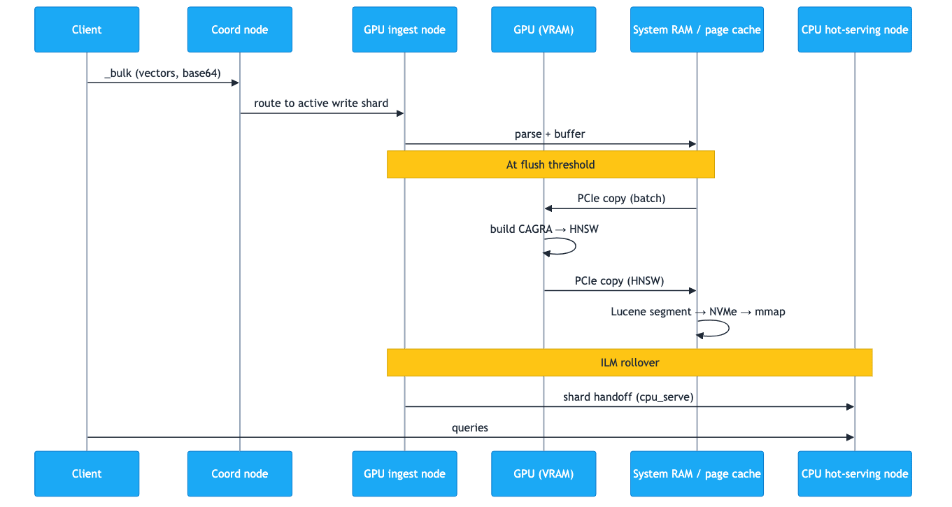
How data flows through Pattern B, end to end
In Pattern B, vectors flow from the client to a GPU ingest node, where cuVS builds the HNSW segment on the GPU before ILM migrates the finished shard to a CPU hot-serving node. The sequence diagram below shows the round-trip for one batch of vectors, followed by the rollover that moves the finished shard to the serving tier:
In step form:
- A client sends a
_bulkrequest with vectors encoded as base64 strings (recommended for throughput). - The coordinating node routes the request to the GPU ingest node that owns the active write shard.
- The GPU ingest node's JVM parses the request, queues vectors in the write buffer.
- At flush threshold, the cuVS plugin batches vectors and copies them from system RAM to GPU VRAM via PCIe.
- The GPU constructs a CAGRA graph in VRAM and converts it to HNSW format.
- The HNSW data is copied back to system RAM via PCIe.
- Lucene writes the segment file from system RAM to local NVMe.
- The segment is memory-mapped into OS page cache (system RAM) and is now queryable.
- After the configured rollover threshold (time or size), ILM rolls the index over and creates a new write index on the GPU ingest tier.
- The rolled index's allocation requirement changes from
gpu_ingesttocpu_serve, and Elasticsearch's shard allocator migrates the shards to CPU hot-serving nodes over the network. - CPU hot-serving nodes memory-map the received segments into their page cache and begin serving queries.
- The GPU ingest node's page cache is released as shards leave, freeing it for the next write cycle.
At no point does query traffic touch the GPU ingest nodes. At no point does the GPU need to hold more than one batch of vectors in VRAM. The GPU is busy during steps 4–6 and idle otherwise. System RAM is in the path on both sides of the GPU: as the staging area for PCIe transfers, and as the persistent page cache for serving.
Adding a BBQ cold tier with requantization
Pattern B extends to a BBQ cold tier for long-retention corpora. BBQ delivers roughly 8x compression over int8, shrinking the cold tier's RAM and disk footprint dramatically. The ILM policy adds a phase that reindexes the int8_hnsw data into a new index configured with bbq_hnsw:
In practice, the requantization happens via a separate reindex job triggered alongside the cold-phase transition. BBQ delivers roughly 8x compression over int8 (and ~32x over float32), so the cold tier's RAM and disk footprint shrinks dramatically.
Note that BBQ is a CPU-only quantization path. bbq_hnsw is not supported by cuVS in Elasticsearch as of 9.5. This is why the GPU ingest tier builds with int8_hnsw and the BBQ conversion happens later, on CPU warm or cold nodes. There is no GPU dependency on the cold path.
Which pattern should you choose?
For most production clusters with five or more data nodes, Pattern B is the better default. Pattern A is the right choice for proof-of-concept deployments and small clusters where operational simplicity matters more than cost.
| Factor | Pattern A (combined) | Pattern B (dedicated GPU ingest) |
|---|---|---|
| Cluster size | Fewer than ~5 data nodes | 5+ data nodes |
| Operational complexity | Lower | Higher (ILM + allocation routing) |
| GPU pod system RAM | 128–192 GB | 64 GB |
| GPU utilization | GPU idle during queries | GPU idle between flushes, but node is not serving queries |
| Hardware cost | Higher (each GPU node needs query-serving RAM) | Lower (GPU ingest nodes are lean) |
| ERU impact | Higher | Lower |
| Best for | POC or edge deployments | Production at 5+ data nodes |
For most production deployments, Pattern B is the better default. The operational complexity is modest (the ILM policy and allocation attributes shown in this post are the entire implementation), and the savings in GPU-node RAM and ERU are material.
Getting started with NVIDIA cuVS GPU vector indexing
GPU-accelerated vector indexing with NVIDIA cuVS is available in technical preview for Elasticsearch 9.3 (self-managed Enterprise) and is targeted for general availability in Elasticsearch 9.5.
Requirements:
- Elasticsearch 9.3+ with Enterprise subscription
- NVIDIA Ampere architecture GPU or newer (compute capability ≥ 8.0), minimum 8 GB VRAM
- CUDA 12.x and cuVS runtime libraries (refer to the Elastic support matrix for exact supported versions)
- Java 22 or higher on the GPU node
- Linux x86_64
- Fast local NVMe (network-attached storage is not recommended)
For teams weighing this against FAISS or a dedicated vector database like Milvus or Pinecone, the operational pitch is the same single platform, same ATO, same ops model, with GPU-accelerated ingest layered onto an existing Elasticsearch cluster. The broader Elastic and NVIDIA partnership context is in Elastic and NVIDIA together unlock next generation enterprise AI search.
Start with Pattern A on a single GPU node to validate throughput on your corpus. Once you have confidence in the numbers, move to Pattern B with the ILM policy above, scale the CPU hot-serving tier to match your query SLA, and let the GPU ingest tier do the one thing it is built for: building HNSW graphs at 12x the speed of CPU.
For the cuVS benchmark methodology and results, see [Up to 12x faster vector indexing in Elasticsearch with NVIDIA cuVS]. For the broader Elastic and NVIDIA partnership, see [Elastic and NVIDIA together unlock next generation enterprise AI search].
常见问题
Why is Elasticsearch vector indexing slow on large corpora?
HNSW graph construction is CPU-bound and dominates indexing time at scale. Adding the NVIDIA cuVS plugin moves the graph build to the GPU, where it runs up to 12x faster on the benchmark hardware. For corpora in the hundreds of millions of vectors, that turns weeks-long indexing campaigns into days.
How do I deploy GPU vector indexing in Elasticsearch without serving queries on the GPU node?
Use a two-tier architecture: GPU ingest nodes with the cuVS plugin and 64 GB of RAM build HNSW segments and own the active write shard. An ILM rollover then migrates the finished shard to a CPU hot-serving tier with 192 GB of RAM, which handles all queries. A custom node attribute, tier_function, controls which nodes receive new writes versus migrated shards.
Can the Elasticsearch `dense_vector` field use NVIDIA cuVS for GPU acceleration?
Yes, on self-managed Enterprise Elasticsearch 9.3 and later, with the cuVS plugin installed on a node that has a supported NVIDIA GPU. You must explicitly set index_options.type to int8_hnsw or hnsw on the dense_vector field, because the default bbq_hnsw in 9.1 and later is not GPU-accelerated by cuVS.
How much RAM does a GPU vector indexing node in Elasticsearch need?
A GPU ingest node only holds the currently-writing shard, so roughly 60 GB total is enough (32 GB JVM heap, 10 GB CUDA runtime and pinned PCIe buffers, 10-15 GB page cache, 5 GB OS), matching the AWS g6.4xlarge benchmark hardware. CPU hot-serving nodes that hold the accumulated HNSW corpus need 128-192 GB depending on shards per node.
Why is my Elasticsearch GPU plugin not accelerating vector indexing even with cuVS installed?
The most common cause is using the default bbq_hnsw index option, which the cuVS plugin does not support. Set index_options.type to int8_hnsw or hnsw in the dense_vector mapping. Also verify the node has a compute-capability 8.0 or higher NVIDIA GPU, CUDA 12.x, and vectors.indexing.use_gpu set to true.
How do I configure ILM to migrate Elasticsearch shards from a GPU build tier to a CPU serving tier?
Set "migrate": {"enabled": false} on the warm phase so ILM does not try to move shards to a data_warm role that does not exist in this architecture, then use an explicit allocate action to route shards to nodes with node.attr.tier_function: cpu_serve. The full policy structure and index template are in the post.
Should I use Elasticsearch with NVIDIA cuVS or a dedicated vector database?
If you already run Elasticsearch for search, observability, or security, adding cuVS lets you serve agentic AI workloads on the same platform without a second data store or a separate operational model. cuVS also runs entirely on local hardware, which matters in air-gapped, sovereign, and on-premises environments where hosted vector databases are not an option.
相关内容
2026年5月18日
Agentic AI search with deterministic guardrails in Elasticsearch for safe query execution
Agentic AI search systems often fail when LLMs generate queries directly. Learn how deterministic guardrails and a control plane architecture enable safe, reliable, and governed query execution with Elasticsearch.

2026年5月13日
Ecommerce search optimization using margin and popularity boosting in Elasticsearch
Learn how to optimize ecommerce search using margin and popularity boosting. This blog explains how a governed control plane treats economic optimization in Elasticsearch.

2026年5月11日
Bringing Fire to Elasticsearch: Adding Native Prometheus API Support
Query Elasticsearch directly from Prometheus-compatible clients via native PromQL, discovery, and metadata endpoints. Send data to Elasticsearch with Prometheus Remote Write.

2026年5月11日
Personalizing ecommerce search: Integrating purchase history and user cohorts
Learn how to create a personalized ecommerce search experience in Elasticsearch without breaking governance. This post explains how to boost products a shopper has purchased before and how to activate cohort-specific policies based on user profiles.

2026年5月13日
Elasticsearch Vector DiskBBQ filter search is now 3–5x faster
Learn how Elasticsearch 9.4 makes restrictive filtered DiskBBQ vector search 3–5x faster and more stable by avoiding wasted centroid and postings-list work when selectivity is high.