Results from Machine Learning (ML) anomaly detection jobs that use geographical functions can now be viewed in Elastic Maps. The 8.1.0 release of Elastic Maps can generate a map of the anomalies by location and help you explore new trends in your data.

Elastic Maps is available on Elastic Cloud. You can also download the Elastic Stack and our cloud orchestration products, Elastic Cloud Enterprise (ECE) and Elastic Cloud for Kubernetes (ECK), for a self-managed experience.

In this example, we will use General Transit Feed Specification (GTFS) data. GTFS defines a common format for public transportation schedules and associated geographic information.

About the data

This data is a collection of approximately 2 months of gtfs-realtime data streamed from San Antonio, TX. This data consists solely of the vehicle position updates with each bus position updated approximately every 5 min. The data is sparse during off hours (between 00:00-05:00) each day. Each individual bus follows deterministic, daily patterns. These patterns, for certain buses, follow deterministic seasonality that can vary day-to-day. The data consists of 2,882,527 unique events from 24-Apr-2019 to 13-Jun-2019.

Data provided by VIA Metropolitan Transit.

Creating the anomaly detection job

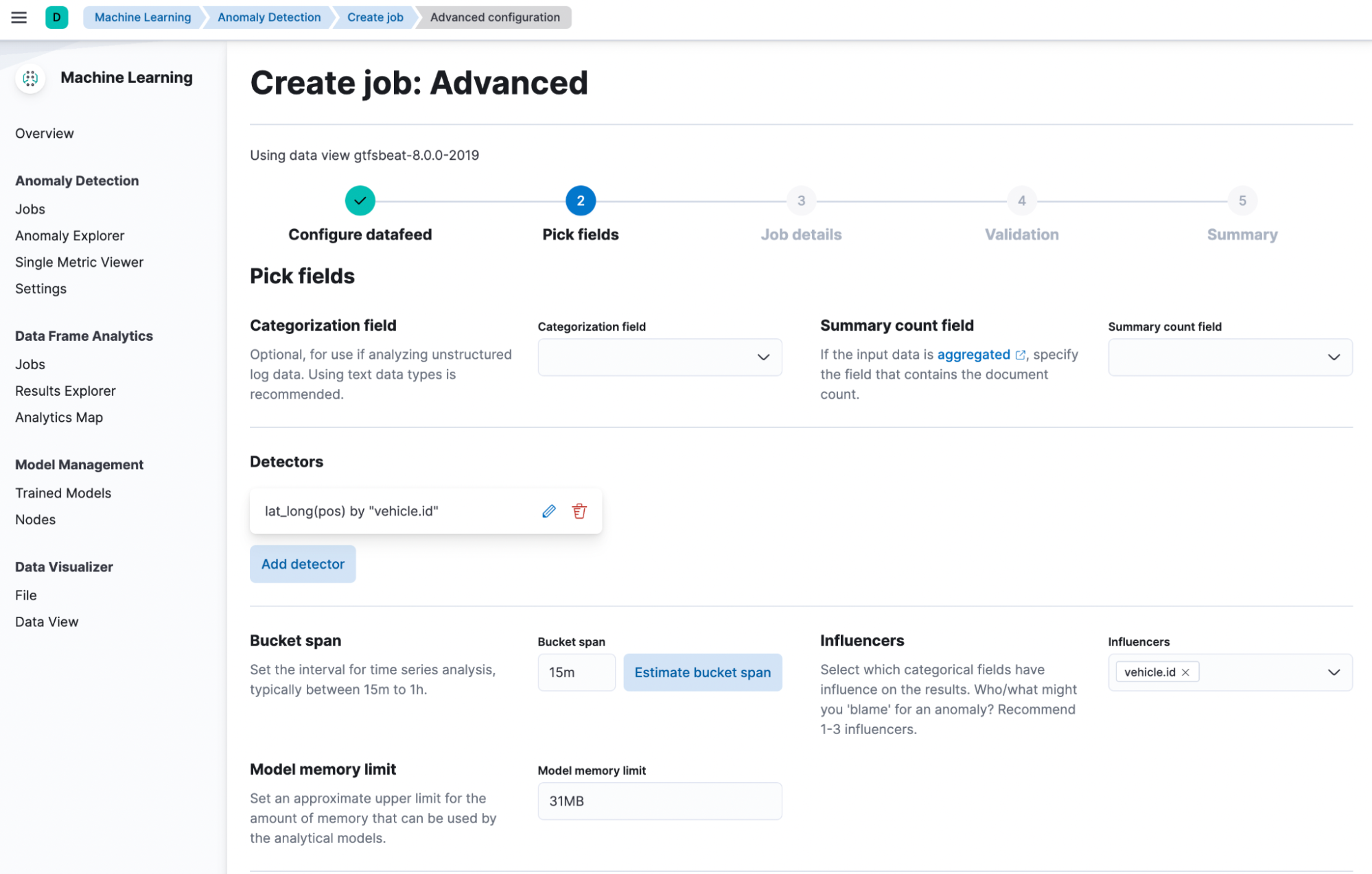
To create an anomaly detection job in Kibana, click Create job on the Machine learning > Anomaly detection page and select the advanced job wizard. Alternatively, use the create anomaly detection jobs API.

Use the  lat_long function in a detector in your anomaly detection job for the pos field (a geo-point field) and set the by field to vehicle.id.

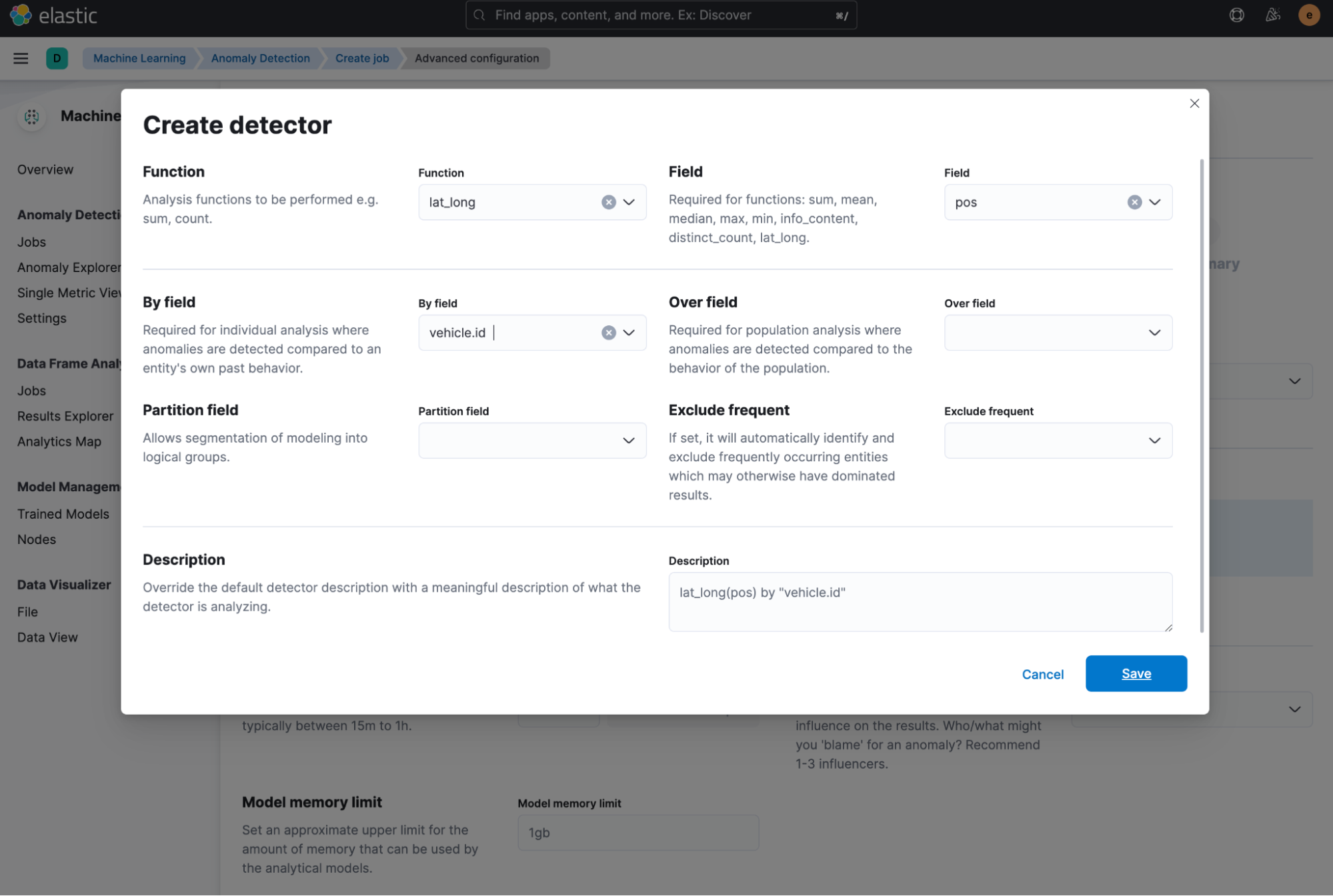
This detects anomalies where the geographic location  (pos) of a vehicle (a bus, in this case) is unusual for that particular bus (vehicle.id). An anomaly might indicate a problem or unforeseen delay.

You should then also select vehicle.id as an influencer for this job. For more information regarding influencers, see the documentation.

Once you’ve created the job and it has produced some results, you can navigate to Elastic Maps to view them.

Mapping anomalies by location in Elastic Maps

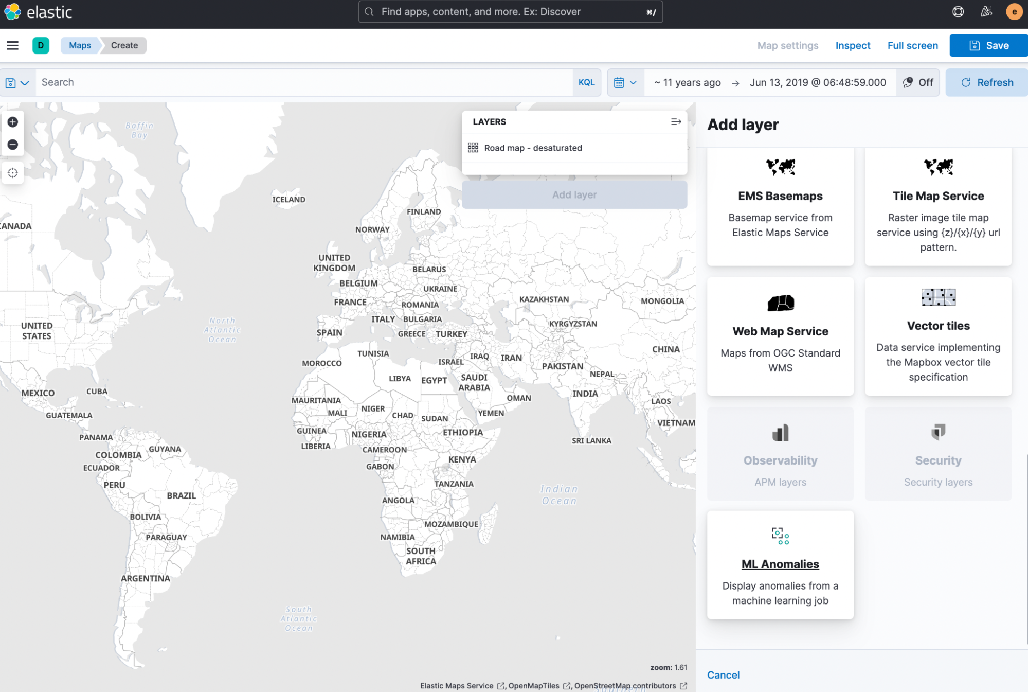
Navigate to Elastic Maps and select Create Map, then select Add Layer. You should see the ML Anomalies layer card option which you can now select.

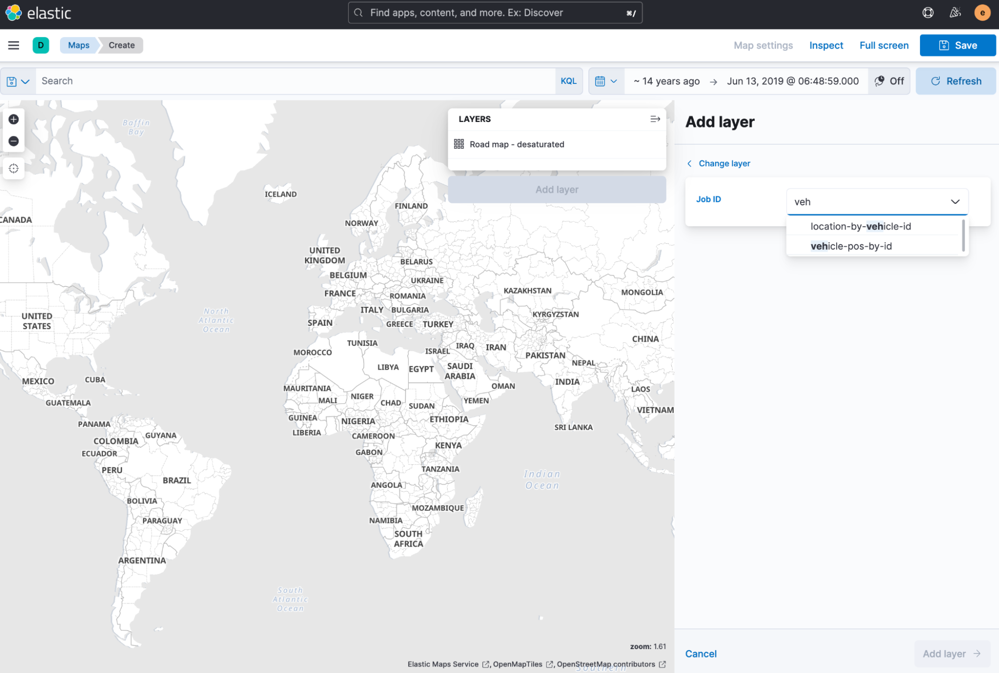
You can now select from a list of jobs - only jobs with geo location data in the results will be in this list. 

Once you have a job selected, notice - in the screenshots below - that you can choose between a few layer options: ‘Actual’, ‘Typical’, and ‘Actual to typical’ . The ‘Actual’ layer is displayed by default until another is selected. This layer displays the actual geographical position of the associated entity on the map.

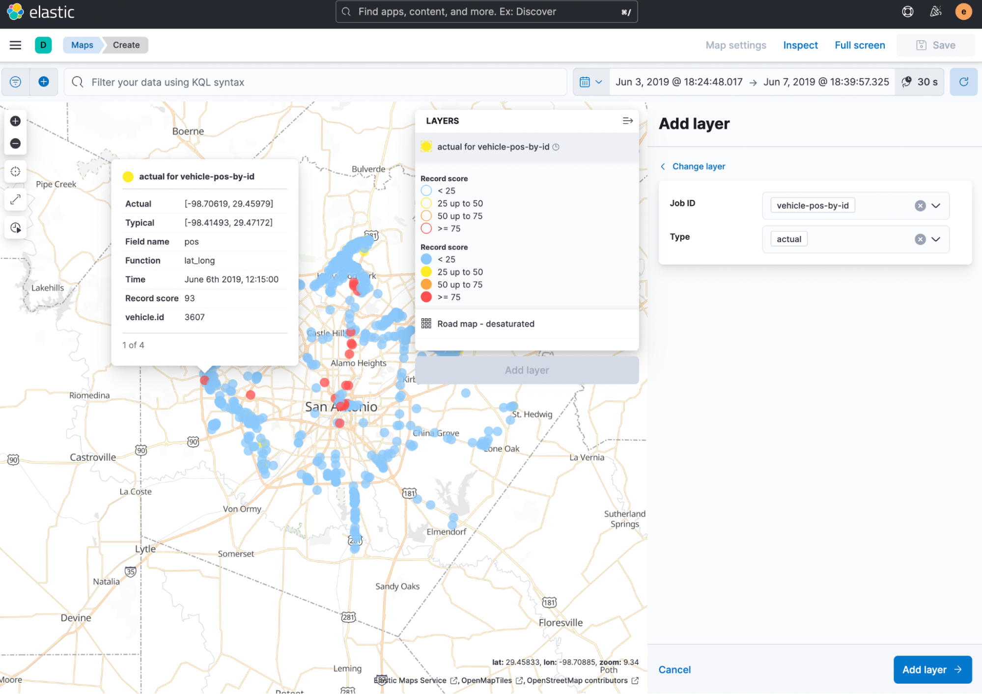
As shown in the expanded legend in the above screenshot, the points are colored according to the severity level of the anomaly - this is determined by the record score of the anomaly. The tooltip for each point will provide more relevant information about the anomaly including the coordinates for both typical and actual positions, record score, and the split field name and value (if there is one).

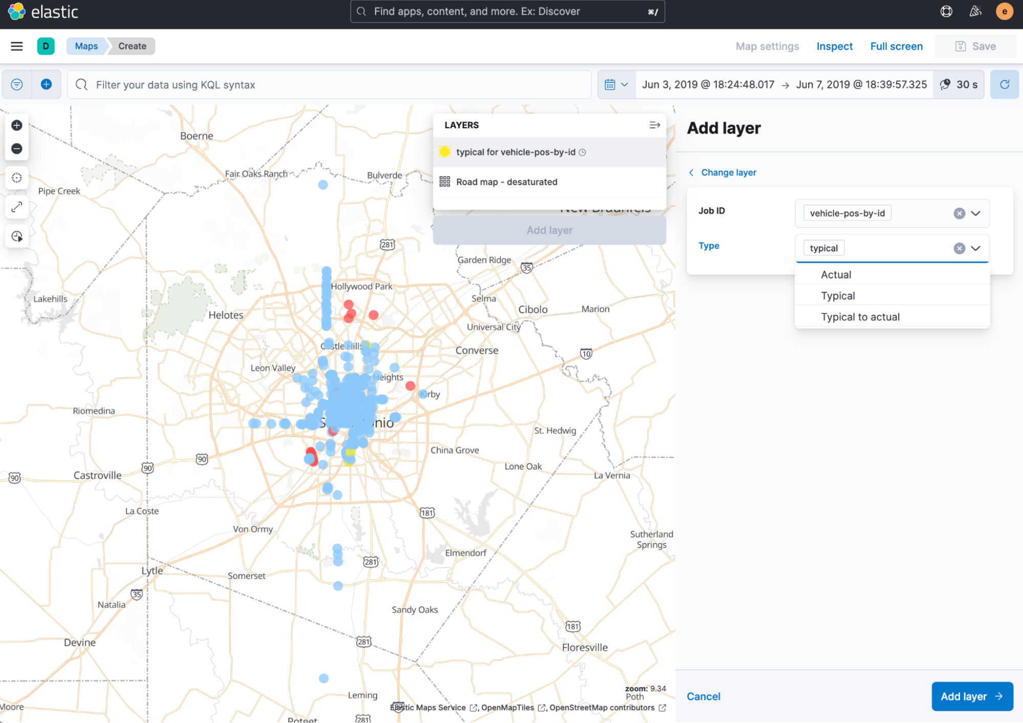
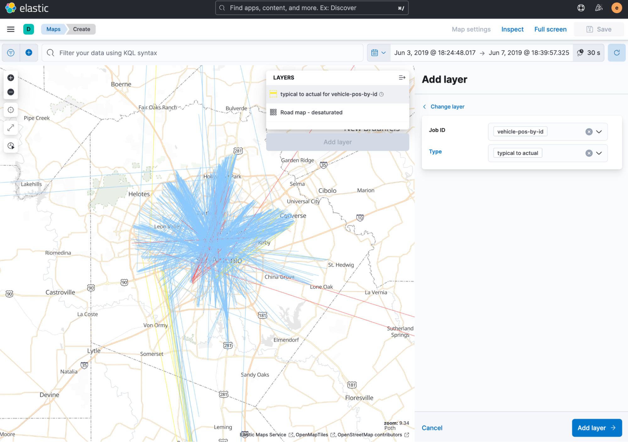
Below, you can see the ‘Typical’ and ‘Typical to actual’ layers in action.

The ‘Typical to actual’ layer connects the typical location, found by the analytical modeling, to the actual location with a line to highlight the difference between these locations.

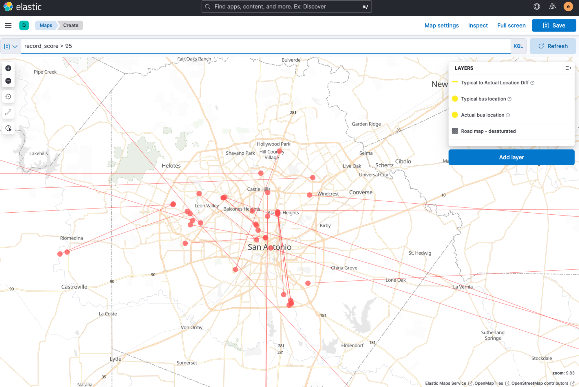
It might be useful to view all three layers at once so you can view a vehicle’s actual location alongside the typical location. This might be a bit overwhelming when you’ve got a lot of data to visualize on the map.

You may only be interested in anomalies for a particular time frame - iin the screenshot above we are limiting the timeframe to the first week of June 2019 - or with a high record score - indicating they are particularly anomalous. In the screenshot below, with all layers showing in the map, we can filter for anomalies with a record score higher than 95.

This allows for a closer look at the buses that are furthest from their typical location for that day and time.

Hovering over one of these points, as shown in the image below, you can see in the tooltip the vehicle id of the particular bus - in this case, it’s 4291.

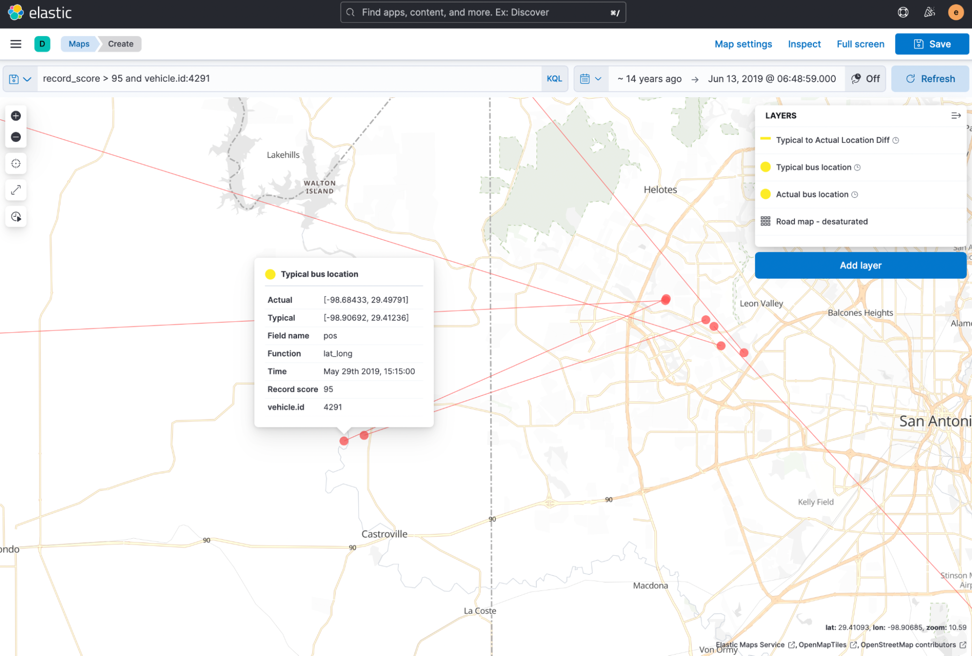
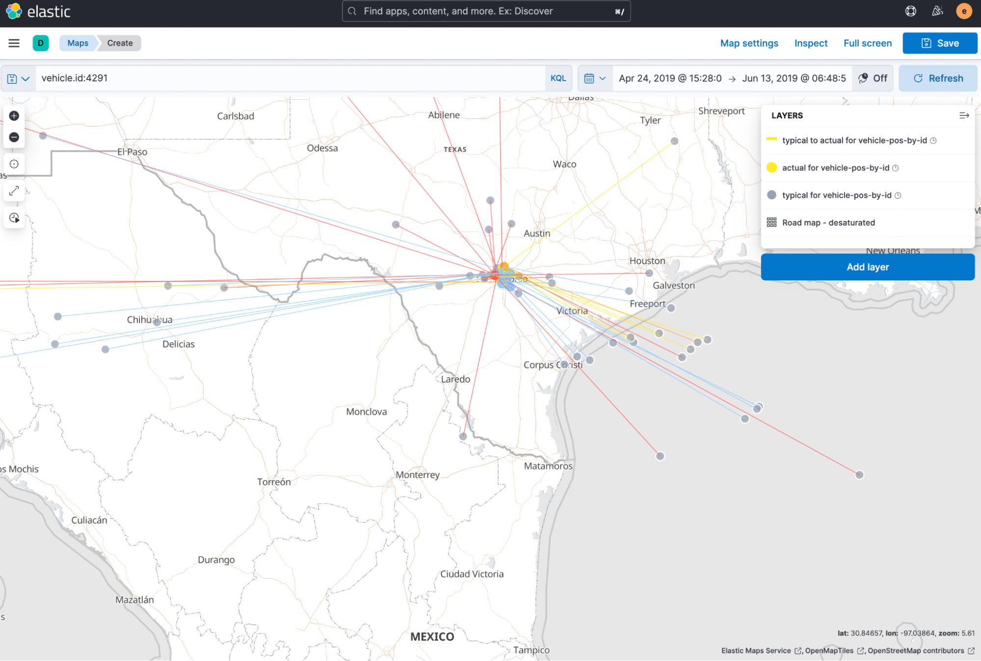
You can narrow the results on the map even further to only view anomalies for that vehicle id.

Now you can see clearly the actual and expected locations for this bus and can investigate further from there.

Link to Maps from Elastic Machine Learning

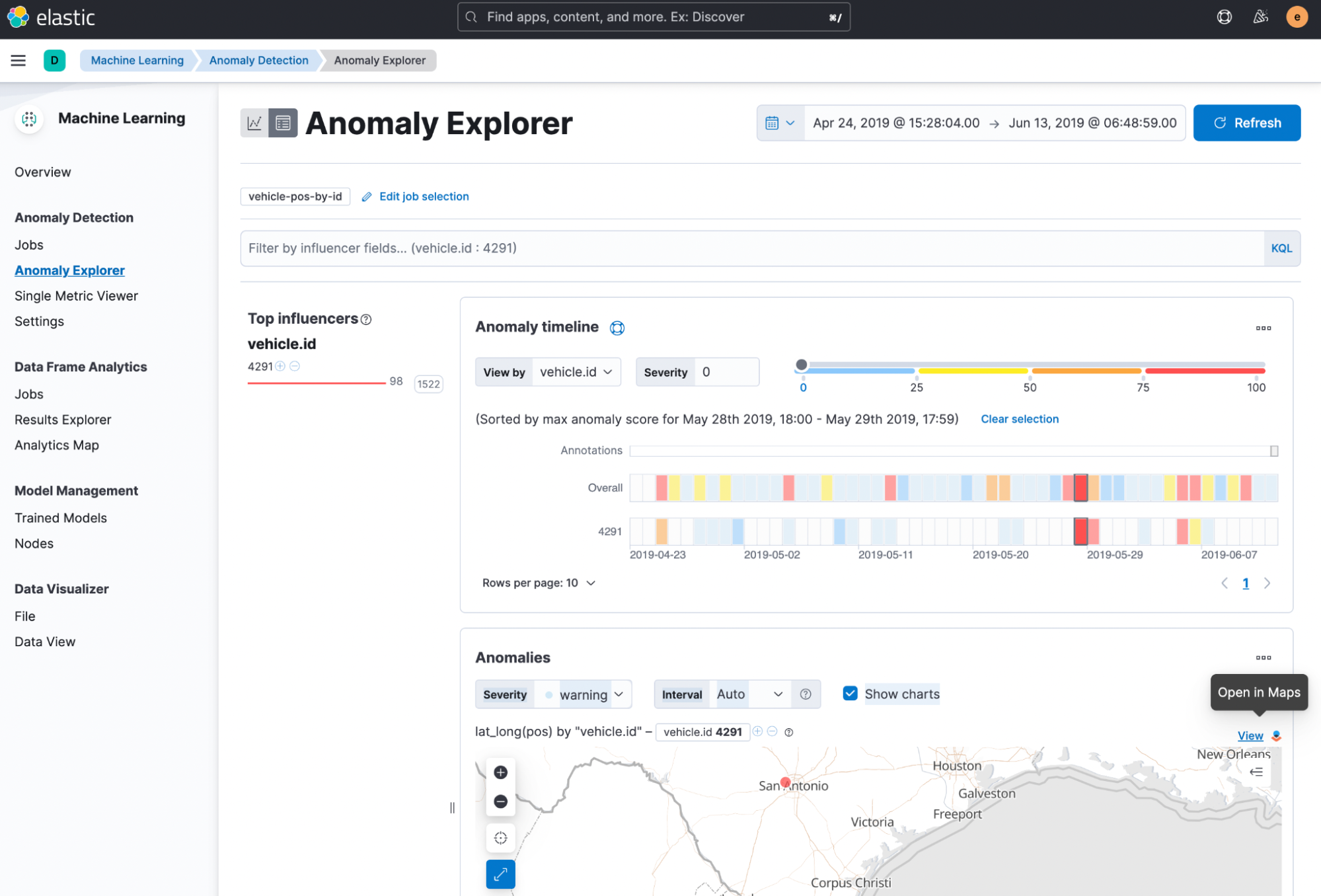
Alternatively, you can now also navigate directly into Elastic Maps from the Anomaly Explorer view in Elastic Machine Learning. This is useful when you’re viewing the results of a job inside the ML app and want to jump directly into Maps with the relevant job and filters already created for you.

In the screenshot below, the swim lane cell for vehicle id 4291 has been selected - you can now select the `Open in Maps` link above the embedded map.

Give it a try

Want to take Elastic Machine Learning and Maps for a test drive? Pick up a free 14-day trial of the Elasticsearch Service, or you can download it as part of the default distribution.